Self-Organizing Maps, or SOM, represent a form of artificial neural network (ANN) employed for unsupervised learning. They facilitate the reduction of data dimensionality while retaining their topological structure, thus offering a robust tool for clustering and data exploration.
Unlike traditional neural networks, self-organizing maps function via competitive learning as opposed to error correction. They incorporate a neighborhood function to preserve the spatial relationships of the data.
Origin of SOMs
Self-organizing maps were introduced in the 1980s by the Finnish researcher Teuvo Kohonen. This is why they are also referred to as Kohonen maps.
Inspired by biological brain mechanisms, they emulate how neurons organize and classify information, forming meaningful structures.
How SOM Works?
The learning process of a Self-Organizing Map relies on multiple steps that transform complex data into an organized and readable representation. Below is a typical, step-by-step operation of a SOM.
1. Initialization of Weights
Before training starts, each neuron in the map is linked to a weight vector, which is initialized randomly. This vector shares the same dimension as the input data and embodies the identity of each neuron prior to adjustment through the learning process.
2. Selection of an Input Sample
During each iteration, an input vector is randomly selected from the training dataset. This vector signifies a data point that the SOM must learn to organize on the map.
3. Identification of the Best Matching Unit
Once the sample is chosen, the algorithm identifies the neuron whose weights are closest to this input vector. This proximity is determined using the Euclidean distance between the input vector and the neurons. The closest neuron is pinpointed as the BMU (Best Matching Unit).

4. Updating the Weights of the BMU and Its Neighbors
After locating the BMU, the algorithm adjusts its weights to align more closely with the input vector. Neighboring neurons are also updated, albeit to a lesser extent.
The extent of this update is influenced by two primary factors:
- The learning rate (denoted as α or alpha) : Alpha governs the speed of adjustment for the neurons’ weights. It diminishes over iterations to prevent abrupt changes.
- The neighborhood function : The update affects neurons around the BMU, with an impact that lessens with distance. A common choice is the Gaussian function.
This phase enables the BMU and its neighbors to gradually align with the characteristics of the data while maintaining the topological integrity of the relationships between data points.
5. Reduction of the Learning Rate and Neighborhood
As the iterations proceed, the learning rate and the neighborhood size decrease. This reduction allows for precise fine-tuning of weights in the final training stages and ensures effective organization of the data on the map.
- Initially, the neighborhood is extensive, enabling the entire map to organize globally.
- Gradually, the neighborhood contracts, refining the map and stabilizing the formed clusters.
6. Convergence and Stabilization
The training continues until the map achieves a stable state where the neurons’ weights exhibit minimal change from one iteration to the next. In this stage, each neuron corresponds to a specific region of the input data.
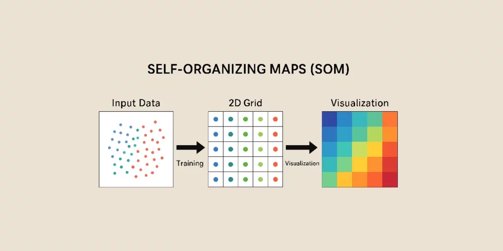
7. Inference and Visualization of Results
Once the SOM is trained, it can organize new data and facilitate visual analysis. The distance between an input vector and the neurons’ weights helps determine the positioning of new data on the map.
A popular method for visualizing SOMs involves assigning colors to different map regions. Darker colors indicate a higher concentration of data.
Clusters of similar data become apparent on the map, providing an intuitive visualization of the interrelationships between various categories.
Advantages and Disadvantages of SOM
SOMs offer several significant advantages. They enable dimensionality reduction while maintaining topological organization. Their intuitive graphical representation aids the visualization and interpretation of complex datasets. They are commonly used for clustering, even without prior knowledge of the data classes.
However, SOMs have certain drawbacks. They do not adapt well to purely categorical or mixed data (except with proper encoding), which makes it challenging to follow a logical representation space. Their training time may be lengthy, and their effectiveness hinges on accurate parameter tuning.
Applications of SOM
SOMs find application in diverse fields to organize and analyze data. For instance, in the marketing sector, they assist in grouping customers based on purchasing behavior to optimize business strategies.
For dimensionality reduction, they aid in the mapping of high-dimensional data, facilitating a better understanding of internal data relationships.
In anomaly detection, they are utilized to identify fraudulent transactions by pinpointing data points that deviate from predefined clusters.
For data visualization, they enhance understanding of populations and relationships between different parameters. By converting a complex dataset into a 2D representation, they allow for rapid identification of trends and invisible patterns in raw data tables.

Conclusion
SOMs are a formidable tool for unsupervised learning in cluster analysis, dimensionality reduction, and data visualization. They do have limitations regarding training time and adaptation to mixed data. They are employed in fields such as finance, marketing, healthcare, and image analysis. Their capacity to unveil hidden structures in data renders them an indispensable choice for exploring unlabeled data.


