Data analysis can be seen as an experimental science, where properties are demonstrated after being observed, and codes are heuristically established to interpret the results. In machine learning and data analysis, dimension reduction plays an essential role in simplifying complex data sets.
The basic idea behind dimension reduction is to represent multi-dimensional data in a much lower-dimensional space, while retaining the important and relevant information.
Before delving into more mathematical detail, it’s important to understand some key terms.
The vocabulary of dimension reduction
- Dimension space: number of characteristics or variables that describe an object in a dataset. For example, a dataset of characteristics about people might include variables such as age, income, address, gender and level of education. This defines a five-dimensional space.
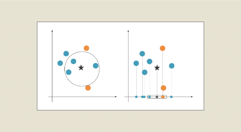
- Projection involves transforming data from a high-dimensional space to a low-dimensional space using dimension reduction techniques. This transformation enables data to be represented more compactly, while retaining important information.
- Orthogonality is a mathematical property in which two vectors or two spaces are perpendicular to each other. In the context of dimension reduction, orthogonality is often used to describe variables or components that are decorrelated from one another.
If the data is represented in a table, dimensionality is reduced by reducing the number of columns. If our dataset is composed of more than 3 variables, the higher the dimension, the more difficult it is to visualize. For example, it’s not possible to visualize a dataset with 13 attributes, but it is possible with just 2 or 3. The aim is therefore to project these data onto the 2 or 3 most important axes in terms of information content, in order to keep the data representation as close as possible to that of high-dimensional data.
A very simple example: suppose we have a dataset containing information on students, comprising the following 5 variables, and each student is represented by a row in the dataset, with each variable corresponding to a column.
| Student | Age | Height | Weight | Math | Science |
|---|---|---|---|---|---|
| Student 1 | 18 | 165 | 60 | 85 | 90 |
| Student 2 | 20 | 170 | 65 | 75 | 80 |
| Student 3 | 19 | 175 | 70 | 90 | 95 |
| Student 4 | 22 | 180 | 75 | 80 | 70 |
After applying PCA to reduce the dimension, we could obtain a new dataset with fewer variables, for example, by retaining only the first two principal components. This would give us the following dataset:
| Student | Principal Component 1 | Principal Component 2 |
|---|---|---|
| Student 1 | 0.23 | -0.12 |
| Student 2 | -0.12 | 0.10 |
| Student 3 | 0.30 | 0.25 |
| Student 4 | -0.41 | -0.23 |
This data set can be easily represented on a 2-dimensional graph:

Find out more about Principal Component Analysis (PCA)
One of the most commonly used methods is Principal Component Analysis (PCA). PCA seeks to find the principal directions in the data that explain most of the observed variance. To do this, we use the notion of covariance.
Let’s represent our data set, made up of n observations (samples) and p variables (characteristics), by a matrix X of size n x p. Before applying PCA, it is often recommended to standardize the variables so that they have zero mean and unit variance, so that variables with different scales don’t dominate the analysis.
We calculate the covariance matrix of X, which we denote C. This matrix measures the linear relationships between variables. It is calculated using the following formula: C = 1/nXT X
We are looking for the eigenvectors of the covariance matrix C. Eigenvectors are directions in the space of variables that describe the variance of the data. Eigenvectors are normalized so that their norm is equal to 1.
We order these eigenvectors in descending order of their associated eigenvalue: ν1 associated with λ1, ν2 associated with λ2 and λ1≥λ2 and so on. The higher the eigenvalue, the greater the variance explained by the corresponding direction.
We choose a number k of principal components (often 1, 2 or 3) to keep and select the first k eigenvectors (ν1, ν2, … , νk). These eigenvectors form an orthonormal basis in the new reduced-dimensional space. Thus, the new variables created are decorrelated. We denote W the matrix formed by these first k eigenvectors.
We now want to project our data into this new space, a basis of which is composed of the vectors (ν1, ν2, … , νk). To project the original data into this reduced-dimensional space, we use the following linear transformation: Y = XW, where Y corresponds to the coordinates of our data following projection.
There are other methods of dimension reduction, the best-known of which are :
- LDA (linear discriminant analysis): linear discriminant analysis is used to identify directions that are decorrelated from one another. It aims to find a linear projection of the data that maximizes the separation between classes while minimizing the intra-class variance.
- T-SNE (t-Distributed Stochastic Neighbor Embedding): T-SNE is a nonlinear dimension reduction method for representing high-dimensional data in a reduced-dimensional space (typically 2D or 3D). For more details, read this article. T-SNE is particularly well suited to visualizing complex structures and non-linear relationships in data.
Limits and difficulties of dimension reduction
It’s important to note that dimension reduction is a compromise between data simplification and information loss. By reducing the dimension, it is possible to lose some subtle information or specific details. Consequently, it’s crucial to strike the right balance by selecting the appropriate number of principal components that capture most of the relevant information.
Each method has its advantages and limitations, and the choice of method depends on the specific context and objectives of the data analysis.
If you liked this article, you can find out more about these methods in our Data Analyst and Data Scientist training courses.


