The number of expected goals is a new performance indicator that has recently appeared in soccer analysis. This statistic is increasingly used to interpret the physiognomy of a match, but do we really know how to interpret it?
The aim of this article is to present the mathematical realities behind expected goals (xG) as simply as possible. The results presented are taken from a simulation carried out by David Sumpter on the Friends of Tracking youtube channel on Premier League data over an entire season.
What is an expected goal?
What is xG? What does a score of 2.71 to 0.78 in xG correspond to?
For each shot taken in a match, it is possible to assign a probability of the ball finding the back of the net.
For example, a shot from 35 meters will have a very low probability of success (perhaps 5%, i.e. 0.05 xG), whereas a penalty kick will have a good chance of deceiving the goalkeeper (76%, i.e. 0.76 xG). By adding up the expected goals of all the shots in a match, we obtain an xG score.
Compared with the classic score, which only counts goals, the advantage of xGs is that they are calculated over a greater number of events. As a result, they often reflect the physiognomy of a match, and make it possible to identify which team has had the biggest chances.
But how is the expected goals probability calculated?
To understand this, let’s build a simple model of expected goals. Let’s start with the following intuition: the further you are from the goal, the harder it will be to score. In our model, the probability of scoring will be established by considering only the position of the shot.
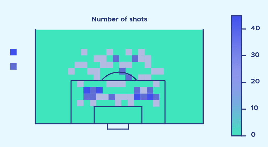
So we’re going to visualize the distribution of shots in 2-dimensional space.
Here’s what we get over a full Premier League soccer season:
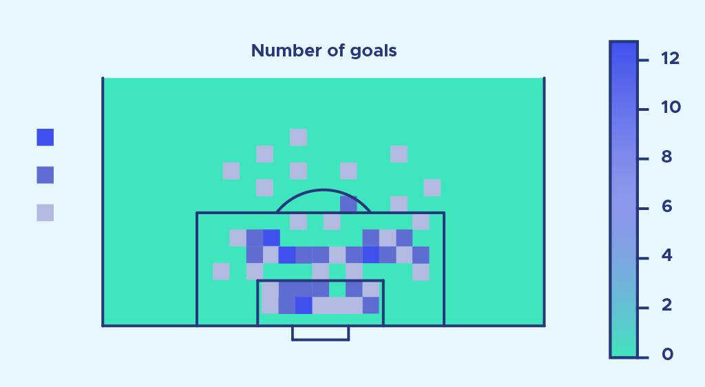
Now let’s compare the number of goals scored:
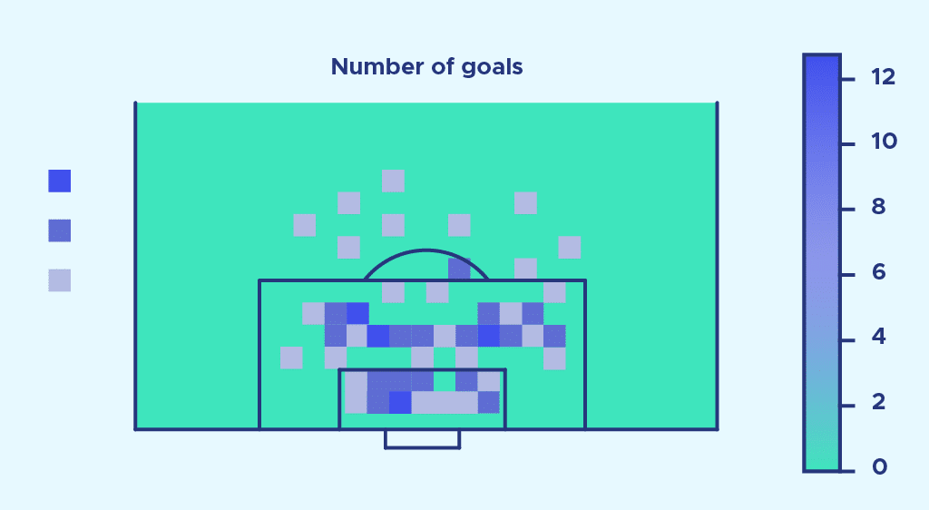
We can see that the number of shots outside the box seems to be proportionally much higher than the number of goals.
Now let’s remember that our aim is to establish a goal probability for each shot. To do this, we calculate the ratio number of goals/number of shots number of goals number of shots for each gridded area of space. This ratio is our probability of scoring. We then display this probability for each zone of the space, and here’s the result:
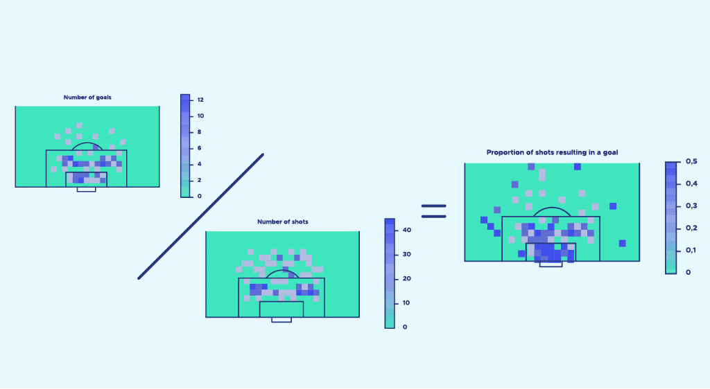
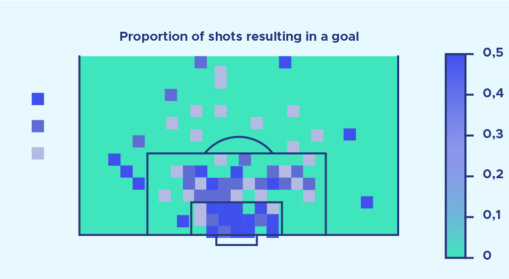
This image is an initial model of expected goals. But as you can see, it’s far from perfect and has many limitations.
The first observation we can make is that the result obtained seems to present anomalies.
Indeed, some very distant areas of space seem to have a very high probability of scoring.
This is due to the fact that the example considered only takes into account shots over a single season, in a single league. Sometimes, there’s just one shot in a very remote area, and that shot is scored – and that’s what we call the magic of soccer. However, if we had carried out our calculations with much more data (several championships over several seasons), the result obtained would have presented less pronounced anomalies.
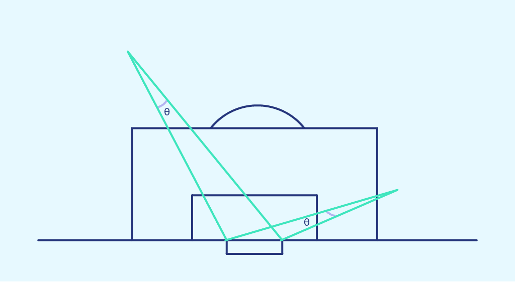
From this generated visualization, we’re now going to try and build a mathematical model that best fits the observed goal frequency. To do this, we’ll study two parameters separately: shot angle and distance to goal.
Shooting angle represents the angle between the two posts at the point of shooting.


This time, we plot the scoring probability obtained previously in each zone of space, as a function of the shooting angle of that zone. We obtain the following point cloud:
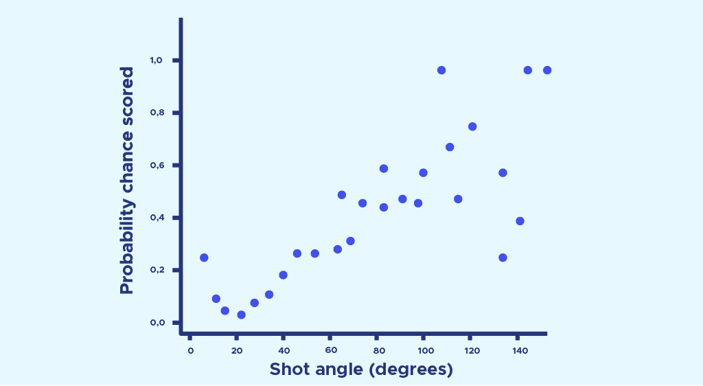
These points can then be approximated by logistic regression using the formula: P(theta) = . We’ve chosen logistic regression rather than linear regression, because the probability of scoring is 1 when the angle approaches 180° and 0 when the angle is 0°.

Now we can do exactly the same thing with the distance :
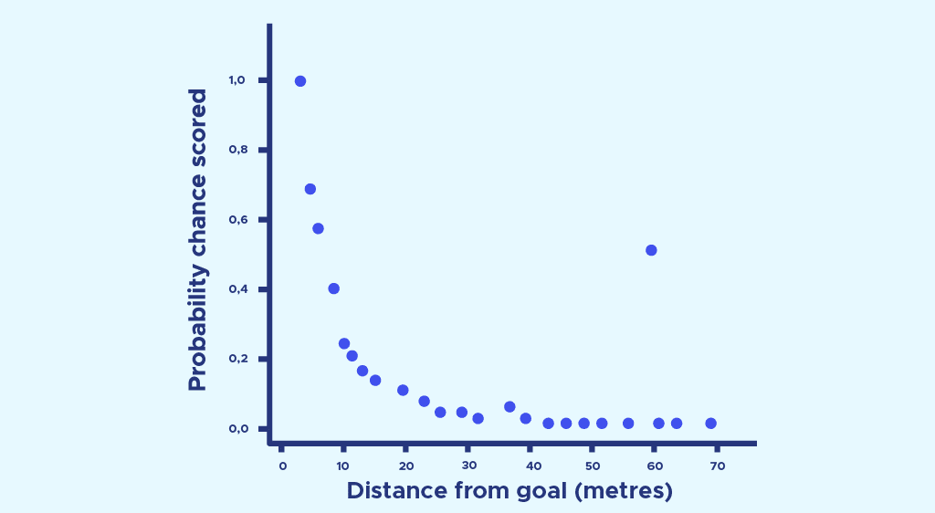
Once again, we run a logistic regression and obtain a probability of scoring as a function of distance:
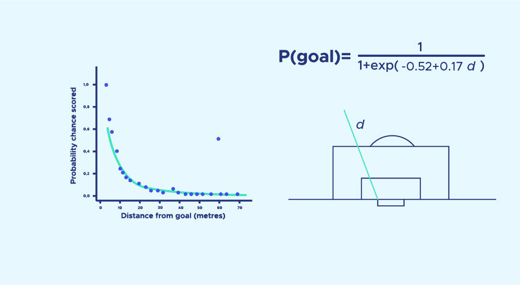
The model isn’t ideal, as the probability of scoring at 0 meters should be equal to 1. It could be improved (for example, by adding a d2to the exponential), but let’s start with this first approximation.
These 2 mathematical models, one based on angle and the other on distance, predict our experimental scoring probability quite correctly. However, they are not ultra-precise.
To improve the accuracy of our mathematical model, this time we take into account the impact of these 2 dimensions simultaneously.
We do this by means of a multivariate regression, but this is a little beyond the theoretical scope of this article. The result that emerges from this bivariate regression is as follows:
This mathematical model takes into account both the angle and distance of the shot. It is designed to be as close as possible to the reality of observed goals. It is now much more general, has fewer anomalies and seems to be closer to reality. Based on this model, it is now possible to assign a probability of scoring to the next shots taken, depending on the area of the shot.
Conclusion
You’ve seen how to build an expected goals model using angle and distance. This model can be used to draw initial conclusions for players. For example, we realize that it’s difficult to score when the shot is off-center, and that a backward pass might be more appropriate.
On the other hand, our model is far from perfect. Its first flaw is that it is based on data from a single championship in a single season. Its second flaw is that we’ve only taken angle and distance into account. More elaborate models will take into account the contact zone of the shot (head or foot), the position of the defenders at the moment of the shot, the type of action (placed attack, counter-attack), the choice of foot (good or bad) and many other parameters.
If there’s one thing to remember from this article, it’s that expected goals are constructed to best match the frequency of goals observed as a function of a multitude of parameters. A probability of scoring remains a probability. It will prove true on average over the long term if correctly constructed, but in a single match anything is possible, and that’s what makes this sport so magical.
If you’re interested in football-related data analysis, we recommend you look at the “MPG, le soccer dans toute sa data” , a project developed in the DataScientest studio.


