
Time series analysis is a crucial methodology in many fields, such as finance, economics, meteorology and biology.
Among the various approaches available, the SARIMAX (Seasonal Autoregressive Integrated Moving Average + exogenous variables) model stands out as a powerful tool for modeling and forecasting both trends and seasonal variations in temporal data, while incorporating exogenous variables into the analysis to improve prediction accuracy.
In this article, we’ll dive into the basics of the SARIMAX model, examine its key components and explore its practical application.
The foundation: the ARIMA model
To fully grasp the essence of the SARIMAX model, let’s start by exploring the basics of the ARIMA (Autoregressive Integrated Moving Average) model. ARIMA is a powerful statistical technique for modeling and forecasting time series. It is based on three key components: autoregression (AR), moving average (MA) and integration (I).
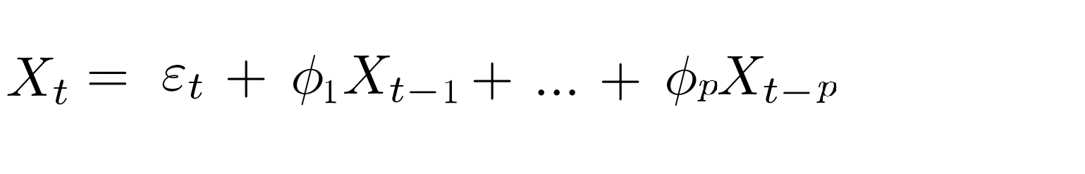
Autoregression (AR) takes into account past values of the time series to predict current values. It is characterized by an order generally noted p. Autoregression consists of performing a linear regression on the last p values of the time series in order to predict the current value:
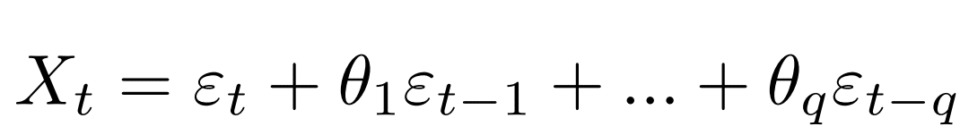
- The moving average (MA), on the other hand, tackles past errors in predictions. It is characterized by an order generally noted q. The moving average consists of performing a linear regression on the last q error values in order to predict the current value:
The combination of autoregression and moving average is the ARMA model. This model is effective on stationary time series. To apply this to any time series, we use the Integration (I) component of the ARIMA model.
- Integration (I) is used to make the time series stationary, by differentiating the values to facilitate modeling. Indeed, most time series can be made stationary after a number of differentiations.
The ARIMA model is then characterized by three coefficients: its autoregression order p. Its integration order d, which corresponds to the number of differentiations required to make the time series stationary. If the series is already stationary, the coefficient d to choose would be zero. Its moving-average order q.
Once these coefficients have been given to the ARIMA model, it will train on the data to find the optimum regression coefficients in the autoregression and moving average to make consistent predictions.
Expanding towards SARIMA: foray into seasonal variations
When temporal data show seasonal variations, the SARIMA model takes over the scene. The term “Seasonal” is added to ARIMA to indicate that this model can capture patterns that repeat at regular intervals.
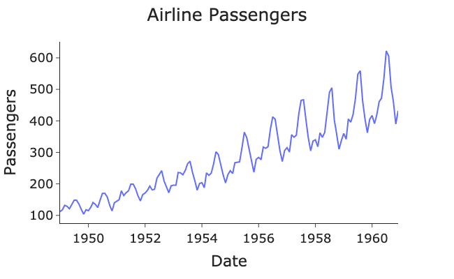
Seasonal variations can occur over short periods, such as a company’s monthly sales, or over longer periods, such as climatic data. By incorporating a seasonal component (S), the SARIMA model can model these recurring patterns and improve forecasts. You can see an example of a non-stationary time series showing seasonality in the graph below, which represents the evolution of an airline’s annual passenger numbers.
The revolution: SARIMAX and covariates
While the SARIMA model already offers a powerful method for modeling seasonal time series, there may be external factors influencing these data. This is where the SARIMAX (Seasonal ARIMA with eXogenous variables) model comes in, opening the door to an even richer analysis.
Covariates, also known as exogenous variables, are external elements that can influence the time series under study. In the context of a company’s monthly sales, covariates might include advertising expenditure, special events or vacations. The SARIMAX model makes it possible to incorporate these covariates into the analysis, thereby allowing for external factors that may affect the trends observed.
SARIMAX model components
The SARIMAX model retains the key components of the SARIMA model while introducing two major elements: the covariates (X) and the covariate component (Z).
- Autoregression (AR): As before, autoregression examines past values of the time series to predict current values.
- Moving average (MA): The moving average continues to model past errors in predictions.
- Integration (I): Integration is always present to make the time series stationary.
- Seasonal component (S): The seasonal component captures variations that recur at regular intervals.
- Covariates (X): Covariates are external variables that can influence the time series.
- Covariate component (Z): The covariate component models the effect of covariates on the time series.
Practical application of SARIMAX with covariates
Let’s take a look at a concrete application of the SARIMAX model to better understand its usefulness. Suppose we have monthly sales data for a company, and monthly advertising expenditure data as covariates.
- Data analysis : Before building the model, it’s crucial to analyze trends, seasonal patterns and the potential influence of covariates on sales. This is the data mining and pre-processing stage.
- Model building: By choosing the ARIMA orders (p, d, q) and the seasonal period (s), we fit the SARIMAX model, taking into account the covariates (in this case, advertising expenditure).
- Validation and forecasting: Evaluate the model’s performance by testing it over a period distinct from the training period. Metrics such as root mean square error (RMSE) give us an insight into the quality of predictions. Once validated, the model is ready to be used for future forecasts.
Conclusion
The SARIMAX model represents a significant advance in time-series analysis by allowing the integration of covariates. By incorporating external variables to enrich the analysis, this model enables us to better understand future trends and predictions. However, as with any methodology, it is crucial to master the model parameters and understand the results to obtain relevant and reliable predictions.
The SARIMAX model with covariates is a valuable contribution to the toolbox of time series analysts, offering a more comprehensive approach to modeling and forecasting data influenced by external factors. Whether anticipating company sales, predicting financial market fluctuations or understanding climatic variations, the SARIMAX model paves the way for more accurate analyses and informed decisions.
By harnessing the model’s powerful covariate integration capabilities, professionals can gain a more holistic perspective on time trends and the factors behind them. Ultimately, the SARIMAX model propels time series analysis to new horizons, enhancing our ability to interpret and anticipate complex temporal behaviors.


