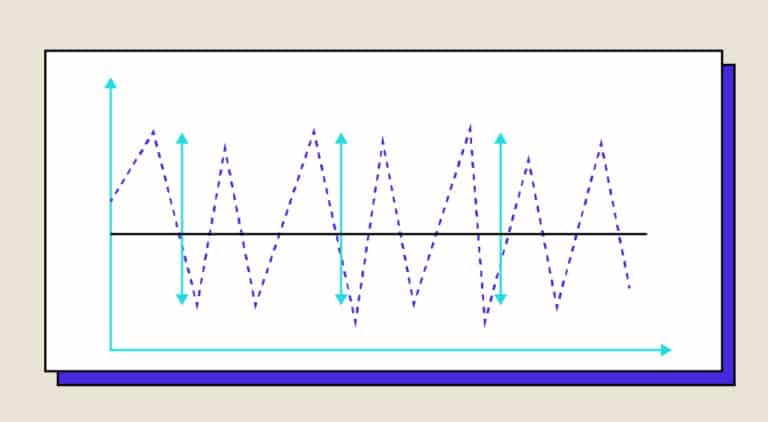
A time series is an array of data showing the evolution of a variable over time. In Python, this is often processed in the form of a Series Pandas indexed by a DateTime. This format makes for easy processing and visualization.
Time series are used in many fields, such as astronomy and meteorology, but are probably most widely used in economics. Think, for example, of company share prices or temperature trends over time.
The ARMA process
AR
A first way of modeling time series is to use the AR or auto-regressive model. This model aims to predict the value of our time series at an instant t using a sum over the previous p instants.
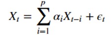
where we have :
- Xt the value at time t
- epsilon t the error at time t
- alpha i the coefficient associated with Xt-i
MA
The MA or moving average process aims to predict the value at time t from the errors of the last q instants.
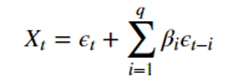
where we have :
- Xt the value at time t
- epsilon t the error at time t
- beta i the coefficient associated with epsilon t-i
ARMA
The ARMA process combines an AR process and an MA process. It is called ARMA(p, q). The exact mathematical formula is as follows:
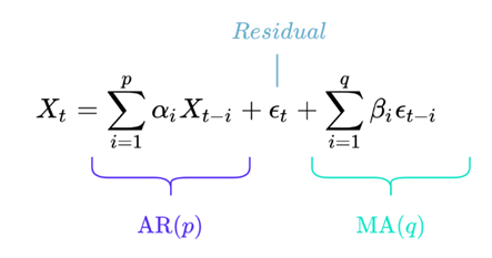
With the same notation as above.
Although this formula can be frightening, it’s actually very simple to understand.
In concrete terms, an ARMA(1, 1) process corresponds to

Limitations of the model
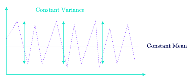
Although this model is very simple and gives good results, it has a few limitations. Firstly, it only gives good results on so-called stationary time series, i.e. with constant mean and variance.
What’s more, it’s difficult to predict the next values at more than t + 1, since we then no longer have any feedback on the error of our model for the MA part.
Python-based study
First analysis
To begin our analysis of the time series, we import the Pandas library and Matplotlib, which will be used for visualization, and read the csv file in which the time series is stored.
In this command line, in addition to the name of the file to be read, the function arguments are :
- parse_dates: this argument tells pandas that the Dataframe contains a date column, and that this is the first column
- index_col: indicates that the index is also the first column
- squeeze: returns a Series instead of a Dataframe
To begin our analysis, we can visualize our time series very simply with the matplotlib.pyplot library, using the following function:
Thanks to this function, we obtain a graph showing the evolution of our variable over time.

Stationarity test
A stationarity test is then performed. The Dickey-Fuller test gives good results quickly and is already implemented in Python in the Statsmodels library.
By importing the function and using it in the following way, we can determine whether our time series can be modeled by an ARMA process:
Here, the terms p and q correspond respectively to the first and last digits of the function’s order argument. The fit method added at the end is used to train the model to determine its parameters on its own.
The summary method is used to check that our model is correct, displaying :
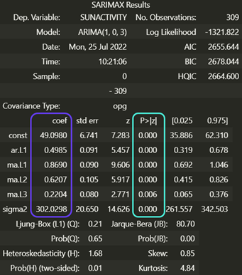
This table may look impressive, but it’s actually very simple to interpret. The column circled in purple corresponds to the model parameters, and the blue column gives the p-value of each parameter. Here we can see that the parameters are good, as the p-value is always less than 0.05. If this is not the case, you can modify p and q to remove unnecessary parameters.
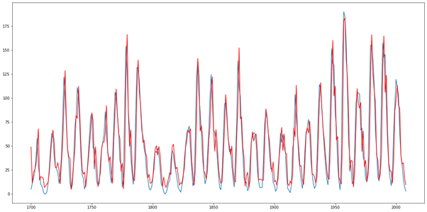
To access and visualize the results, click on :
Our model is shown in red and the actual values in blue:
Conclusion
In conclusion, we’ve succeeded in modeling our time series, but our model does have some limitations, as discussed above. To deal with non-stationary time series, we can use the ARIMA model, which adds differentiation. If our series shows seasonality, i.e. variations at regular time intervals, we’ll need to use the SARIMA model instead. These models and more are covered in our Data Scientist curriculum.


