
A model is said to possess the Markov property if its state at time T depends solely on its state at time T-1. If we observe the states in which the model exists at each moment, we have what is known as an observable Markov model. Otherwise, it is referred to as a hidden Markov model. This article illustrates these models to grasp their functionality and usefulness.
Rigorous Mathematical Definition

In mathematical terms, a sequence of random variables (Xn) taking values in a state space E forms a Markov chain if it adheres to the weak Markov property. This property is articulated by the following equation:
P(X_{n+1} = i_{n+1} | X_1 = i_1, ..., X_n = i_n) = P(X_{n+1} = i_{n+1} | X_n = i_n) This equation implies that the likelihood of moving to the future state i_{n+1} is contingent only on the present state i_n, and not on the entire sequence of previous states.
Key Elements of a Markov Chain
The state space E: this is the set of all conceivable states the system can occupy. In our meteorological example, E = {sun, clouds, rain}.
Transition probabilities: P(X_{n+1} = j | X_n = i) is the probability of transitioning from state i to state j in a single step.
Time homogeneity: if these transition probabilities are independent of time n, the chain is termed homogeneous. This is the most frequently examined scenario.
This mathematical formalization distinctly separates Markov chains from other stochastic processes and serves as the groundwork for their entire theory.
History and Foundations of Markov Chains

Markov chains derive their name from the Russian mathematician Andrey Andreyevich Markov (1856-1922), who presented this concept in 1902 while researching the extension of the law of large numbers to dependent quantities.
Markov initially sought to extend probability limit theorems beyond the realm of independent random variables. His desire was to comprehend how the law of large numbers could apply to sequences of events where each event is dependent on the preceding one, but not on the entire history.
The Conceptual Innovation
Markov’s groundbreaking idea was to model processes where the future is influenced by the past solely through the present. This property, now identified as the “Markov property,” can be intuitively described as: “the past matters only for its influence on the present state.”
Markov himself applied his chains to the analysis of letter sequences in Russian literature, notably in Pushkin’s “Eugene Onegin,” thereby demonstrating the applicability of mathematical concepts to non-mathematical fields.
Modern Developments
Since their conception, Markov chains have undergone extraordinary development and have become an essential instrument in various scientific and technological domains, from statistical physics to contemporary artificial intelligence.
Observable Markov Model
Consider the following scenario:
You are confined in your house on a rainy day, aiming to predict the weather for the next five days.
Not being a meteorologist, you simplify the task by assuming the weather follows a Markov model: the weather on day J depends only on the weather on day J-1.
To further simplify, you consider only three potential weather types: sun, clouds, or rain.
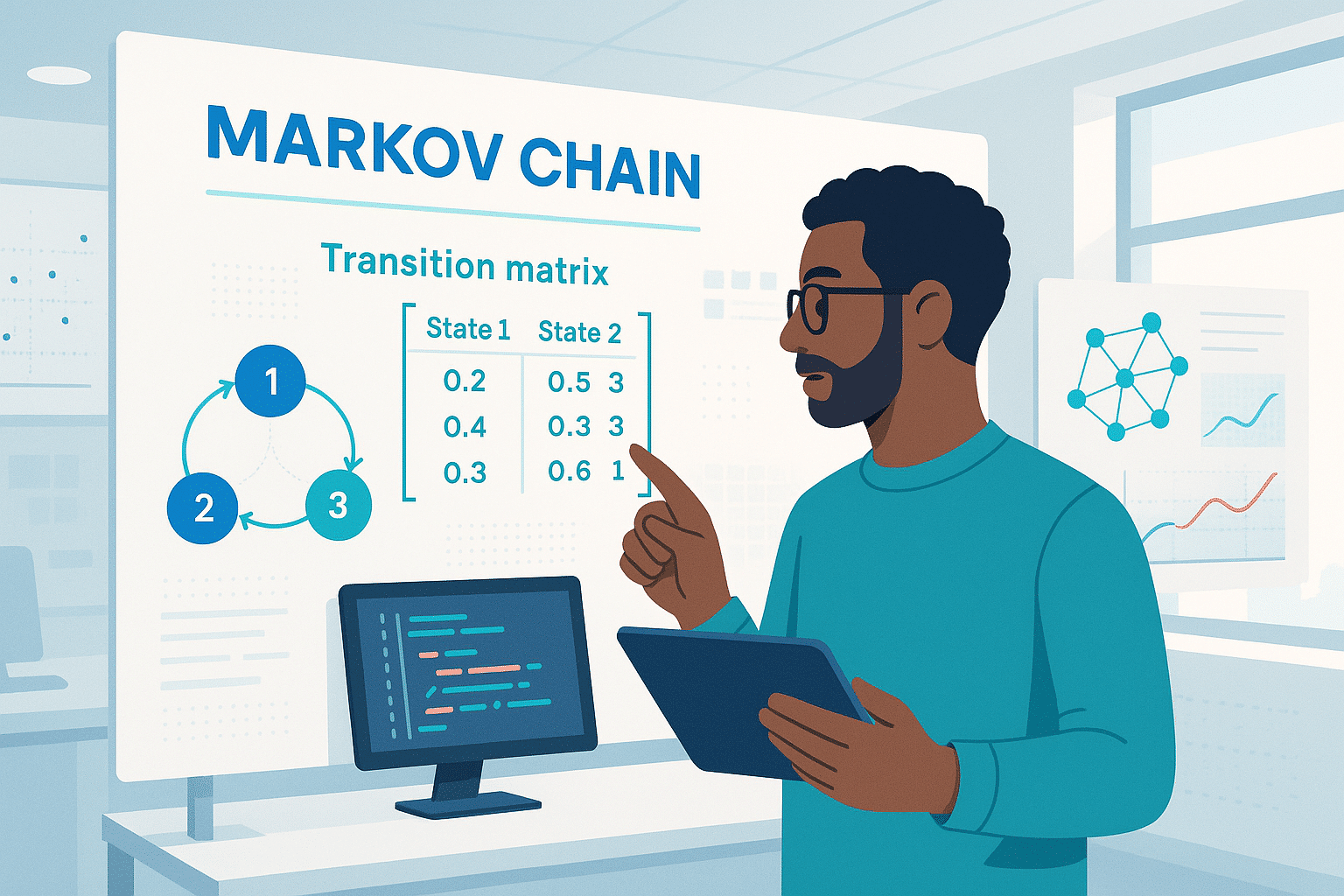
Based on past months’ observations, you create the following transition diagram:
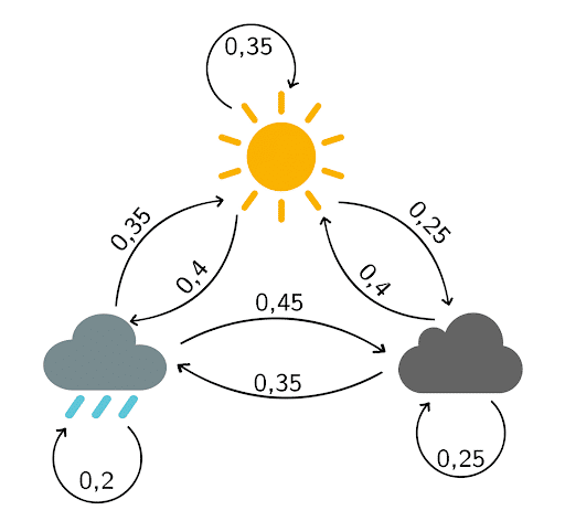
The transition matrix associated is
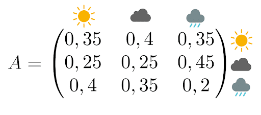
Recall, this matrix is interpreted as follows:
- The probability of fair weather tomorrow given that it is raining today is 35%
- The probability of clouds tomorrow when clouds are present today is 25%
Let’s compute the probability that the weather for the upcoming five days will be “sun, sun, rain, clouds, sun”.
Since the weather of any given day relies solely on the weather of the previous day, it suffices to multiply the probabilities (considering that it is raining today):

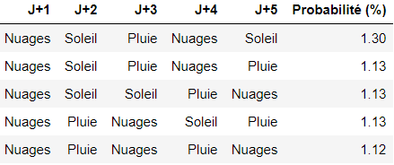
We can calculate this probability for every possible combination and select the one with the greatest likelihood to address the problem.
In our case, here are the five combinations with the highest likelihood of occurring:
Fundamental Properties of the Transition Matrix
The transition matrix used in the prior example contains important mathematical properties that need comprehension.
Matrix Structure
A transition matrix P = (p_{ij}) must meet two essential constraints:
- All entries are non-negative: p_{ij} ≥ 0 for all i,j
- Each row must add up to 1: Σ_j p_{ij} = 1 for all i
This second constraint indicates that from any state, the system must inevitably transition to one state (possibly remaining in the same state).
Matrix Powers and Long-term Predictions
A remarkable property is that P^n (P to the power of n) directly provides the transition probabilities over n steps. Thus, (P^n)_{ij} denotes the probability of moving from state i to state j in exactly n steps.
This property allows for long-term weather forecasts. For instance, if we compute P10, we can determine the transition probabilities over 10 days.
Convergence to Equilibrium
Under specific conditions, the successive powers of matrix P converge to a limit matrix where all rows are identical. This common row represents the system’s stationary distribution; the probability distribution towards which the system gravitates over time, irrespective of its original state.
In our weather model, this implies that in the very long run, the likelihood of experiencing sun, clouds, or rain becomes stable and predictable.
Classification of States in a Markov Chain
Once the transition matrix is determined, it is vital to understand the long-term behavior of each state. This analysis allows for the classification of states based on their dynamic properties.
Transient and Recurrent States
A state is termed transient if, from that state, there’s a non-zero probability of never making a return. A state is termed recurrent if, from that state, a return is certain sooner or later.
In our weather example, should we modify the matrix to include a “storm” state, transitioning only to “rain” without return, then “storm” becomes a transient state.
Absorbing States
A state is absorbing if it is impossible to leave once it is entered. Mathematically, this means p_{ii} = 1 for that state i.
Concrete example: in a life cycle model of an organism with states “juvenile,” “adult,” “senescent,” and “deceased,” the “deceased” state is absorbing as a dead organism cannot change state.
Irreducible Chains
A Markov chain is irreducible if every state can communicate with every other state, meaning it is possible to reach any state from any other state in a finite series of steps.
Our meteorological model is irreducible: the transition from sun to rain (via clouds), from rain to sun, etc., is possible. This property assures the existence of a unique stationary distribution.
Periodicity
A state has a period d if it can only be revisited in times that are multiples of d. If d = 1, the state is termed aperiodic. An irreducible and aperiodic chain always converges to its stationary distribution.
This classification facilitates prediction of the system’s asymptotic behavior and determines which mathematical tools are applicable for analysis.
Stationary Distribution and Convergence to Equilibrium

We previously introduced the notion of convergence to equilibrium. Let’s delve deeper into this fundamental concept.
What is a Stationary Distribution?
A stationary distribution π is a probability vector that stays unchanged by the dynamics of the chain. Mathematically, it fulfills the equation: π = πP, where P is the transition matrix.
In our weather model, if the stationary distribution is π = (0.4, 0.3, 0.3) for (sun, clouds, rain), it implies that in the long term, we will have sun 40% of the time, clouds 30%, and rain 30%, no matter the current weather state.
Existence and Uniqueness
For an irreducible Markov chain with a finite state space, a unique stationary distribution always exists. This outstanding property ensures the system exhibits predictable long-term behavior.
The Ergodic Theorem
The ergodic theorem is one of the most potent results of Markov chain theory. It states that, for an irreducible and aperiodic chain:
- Convergence: Regardless of the starting state, probabilities converge to the stationary distribution
- Law of Large Numbers: The portion of time spent in each state converges to its stationary probability
Concretely, this means if our weather is observed over numerous years, the frequency of each type of weather experienced converges to the stationary distribution probabilities.
Practical Applications of Ergodicity
This property enables the calculation of long-term averages without exhaustive simulation. For example, if a machine is likely operational with a stationary probability of 0.95, it’s understood that it will be available 95% of the time in the long term—a critical factor for industrial scheduling.
Ergodicity also backs the use of Markov chains in Monte Carlo sampling algorithms: by letting the chain operate long enough, one can sample according to the desired outcome distribution.
Practical Exercises to Master Markov Chains

To reinforce your understanding, here are some classic exercises with detailed solutions.
Exercise 1: Ehrenfest Urn
An urn contains 4 numbered balls. At each interval, a number is randomly drawn, and the corresponding ball is shifted to the other urn. The state of the system is the count of balls in the first urn.
Question: Determine the transition matrix and find the stationary distribution.
Solution: The potential states are {0,1,2,3,4}. If urn 1 contains i balls, the probability of transitioning into state i-1 is i/4 (drawing a ball from urn 1), while transitioning into state i+1 is (4-i)/4 (drawing a ball from urn 2).
The stationary distribution is aligned with a binomial distribution: π(i) = C(4,i)/16, hence π = (1/16, 4/16, 6/16, 4/16, 1/16).
Exercise 2: Random Walk on a Graph
A pawn maneuvers on a square with vertices A, B, C, D. At each step, it moves to an adjoining vertex with equal probability.
Question: Is the chain irreducible? Periodic? Calculate the average return time.
Solution:
- Irreducible: Yes, one can move between any vertices
- Periodic: Yes, with a period of 2 (an even number of steps is needed to return to the starting point)
- Average return time: 4 steps per vertex
Exercise 3: Lifespan Model
An organism progresses through the states: juvenile (J), mature (M), senescent (S), deceased (D). The transition matrix reads as:
					J    M    S    D
J [0.6  0.4  0    0  ]
M [0    0.7  0.3  0  ]
S [0    0    0.8  0.2]
D [0    0    0    1  ]
Question: Compute the probability that a juvenile organism reaches the senescent stage.
Solution: The probability needed is 0.4 × (0.3/0.3) = 0.4, as any mature organism inevitably hits the senescent stage.
Exercise 4: Absorption Time
Revisiting the previous exercise, calculate the life expectancy of a juvenile organism.
Solution: Using absorption time equations, the life expectancy of a juvenile approximates 8.33 time units.
These exercises demonstrate theoretical concepts within tangible scenarios and prepare you to model your problems with Markov chains.
Extension to Continuous-Time Markov Chains

To this point, our study focused on discrete-time Markov chains, where transitions happen at regular intervals (day 1, day 2, etc.). In numerous real-world cases, changes between states can occur at any time: this belongs to continuous-time Markov processes.
Fundamental Conceptual Differences
Rather than transition matrices, infinitesimal generators are employed to express instantaneous transition rates. If q_{ij} symbolizes the rate of transition from state i to state j, then the probability of a transition occurring over a small interval dt roughly equates to q_{ij} × dt.
Concrete Example: Call Center
Consider a call center where calls arrive following a Poisson process with a rate of λ = 5 calls/hour, each being attended to in an average of 10 minutes (service rate μ = 6 calls/hour).
States signify the number of calls being handled. Transitions include:
- State n → State n+1 with rate λ (incoming call)
- State n → State n-1 with rate nμ (completion of call handling)
Continuous Chapman-Kolmogorov Equations
The system’s dynamics adhere to the differential equation: dP(t)/dt = P(t) × Q
where Q is the generator matrix and P(t) provides transition probabilities at time t.
Stationary Distribution in Continuous Time
In equilibrium, the condition becomes: π × Q = 0, where π represents the stationary distribution. This equation elucidates flow equilibrium: for each state, the rate of inflow equates to the outflow rate.
Practical Applications
- System Reliability: Equipment failures can arise at any time (rate λ) and require repairs (rate μ). The continuous-time process suitably models these unpredictable phenomena.
- Epidemiology: SIR (Susceptible-Infected-Recovered) models utilize continuous infection and recovery rates for epidemic evolution forecasts.
- Quantitative Finance: Changes in asset prices follow continuous processes, depicted by diffusions (stochastic extensions of Markov processes).
Advantages of Continuous Time
This approach authentically mirrors numerous natural phenomena and frequently permits more elegant analytical calculations. It also bridges to more complex models such as diffusion processes and stochastic differential equations.
Markov Chain Monte Carlo Methods (MCMC)

Markov chains introduce a revolutionary approach in statistical sampling methods, specifically when distributions defy direct sampling.
The Fundamental Principle of MCMC
The brilliant approach is to construct a Markov chain whose stationary distribution is precisely the distribution we aim to sample. Allowing this chain to evolve extensively results in samples that closely match the target distribution.
The Metropolis-Hastings Algorithm
This universal algorithm facilitates sampling any distribution π(x), even when known only up to a normalization constant.
Operating Principle:
- From the current state x_t, propose a new state y according to a proposal distribution q(y|x_t)
- Calculate the acceptance ratio: α = min(1, [π(y)q(x_t|y)] / [π(x_t)q(y|x_t)])
- Adopt y with probability α, otherwise remain at x_t
This process guarantees that the emergent chain’s stationary distribution matches π(x) exactly.
Applications in Bayesian Statistics
In Bayesian inference, often the aim is to sample the posterior distribution of parameters. With data D and parameters θ having a prior π(θ), the posterior distribution follows:
π(θ|D) ∝ π(D|θ) × π(θ)
MCMC enables sampling this distribution even when it lacks a straightforward analytical form, marking a revelation in modern statistical analysis.
Gibbs Sampling
A special case of Metropolis-Hastings for multivariate distributions. Instead of updating all parameters together, each parameter is updated individually while conditioned on others.
This method is especially effective in graphical models like Bayesian networks, where many conditional distributions exhibit simple forms
Convergence Diagnostics
A major challenge in MCMC is determining when the chain has “forgotten” its initial state and is sampling from the true stationary distribution. Diagnostics include:
- Time trace visualization
- Gelman-Rubin criterion (comparison of multiple chains)
- Autocorrelation tests
Contemporary Applications
- Artificial Intelligence: Bayesian neural networks use MCMC to quantify prediction uncertainty — a crucial feature for high-stakes applications.
- Computational Epidemiology: Epidemic spread models with uncertain parameters are calibrated using MCMC based on observed data.
- Quantitative Finance: The estimation of stochastic volatility models and the pricing of complex options rely heavily on MCMC methods.
MCMC perfectly illustrates how a fundamental mathematical concept — Markov chains — has become a revolutionary computational tool for modern data science.
Markov Chains in the Modern Data Science Ecosystem
In the age of big data and artificial intelligence, Markov chains have found new fields of application that go far beyond their original theoretical framework.
Natural Language Processing (NLP)
Markov-based language models were the precursors to modern architectures like GPT. They model the probability of a word based on the preceding ones, enabling:
- Automatic text generation: By chaining transition probabilities, coherent sentences can be produced
- Spell checking: Markov chains detect improbable character sequences
- Text classification: Each class (e.g. spam/non-spam) is modeled with its own Markov chain
Recommendation Systems
Platforms like Netflix or Spotify use Markov chains to model user journeys:
- States: viewed content
- Transitions: probabilities of moving from one item to another
- Goal: predict the next piece of content likely to interest the user
Time Series Analysis in IoT
In the Internet of Things, sensors generate sequential data streams. Markov chains enable:
- Anomaly detection: identifying unusual measurement sequences
- Predictive maintenance: anticipating failures in industrial equipment
- Energy optimization: modeling consumption patterns
Cybersecurity and Fraud Detection
Security analysts use Markov chains to:
- Intrusion detection: model normal user behavior and flag deviations
- Malware analysis: system call sequences reveal malicious software signatures
- Behavioral authentication: identify users based on their navigation patterns
Digital Marketing and Web Analytics
Markov chains enhance the web user experience by enabling:
- Customer journey analysis: understand conversion paths on e-commerce sites
- Sequential A/B testing: assess the impact of changes on browsing behavior
- Marketing attribution: measure the effectiveness of different acquisition channels
Computational Bioinformatics
Beyond classic DNA analysis, modern applications include:
- Gene expression analysis: model the temporal evolution of gene activity
- Genomic epidemiology: trace the spread of viral variants through sequence analysis
- Personalized medicine: predict disease progression using sequential biomarkers
Integration with Machine Learning
Markov chains are increasingly blended with modern techniques:
- Feature engineering: extract explanatory variables from time series data
- Reinforcement learning: Markov decision processes underpin learning by interaction
- Recurrent neural networks: LSTMs and GRUs generalize Markov chains with adaptive memory
These applications show that Markov chains, far from being a purely academic concept, are a foundational methodology for extracting value from sequential data in the modern digital economy.
Hidden Markov Model

We keep the same assumptions as in the previous section.
Now imagine a weather-obsessed psychopath has locked you in a windowless room with only a computer and a lamp. Each day, the lamp lights up in a certain color depending on the weather. Your captor gives you the following observation matrix:
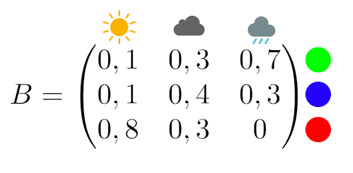
For example, if it’s raining, the lamp has a 70% chance of turning green and a 30% chance of turning blue.
You’ll be allowed to leave if you can determine the weather for the next five days based solely on the lamp’s color. You build a Hidden Markov Model to solve the task.
You stay locked in for 5 days and observe the following lamp colors:
blue, blue, red, green, red
You remember that it was raining the day before you were locked up.
You then write a Python script that returns the most likely weather sequence:

Note: You could also implement the Viterbi algorithm, which would return the most probable sequence — in this case: [‘Cloudy’, ‘Cloudy’, ‘Sunny’, ‘Rainy’, ‘Sunny’].
This prediction approach is interesting but still basic. If you want to learn how to make more impressive predictions — with machine learning algorithms, for example — get in touch with us online to learn more about our data science programs!
Deep Dive into Hidden Markov Models (HMMs)

Our “weather-obsessed psychopath” example offers a playful introduction to HMMs, but these models deserve a more technical breakdown, as they are among the most powerful tools in statistical learning.
Mathematical Structure of an HMM
A Hidden Markov Model consists of three core components:
- Hidden states: the unobservable sequence of states (in this case, the actual weather)
- Observations: what we can measure (the color of the lamp)
- Two probability matrices:
- A, the transition matrix between hidden states
- B, the emission/observation matrix
The Three Fundamental HMM Problems
HMM theory revolves around three central questions:
Problem 1: Evaluation What is the probability of observing a given sequence?
The Forward algorithm efficiently computes this likelihood while avoiding combinatorial explosion.
Problem 2: Decoding What is the most probable sequence of hidden states?
The Viterbi algorithm solves this using dynamic programming. In our weather example, it determines the most likely sequence of weather conditions given the observed lamp colors.
Problem 3: Learning How can the model parameters be estimated from observations?
The Baum-Welch algorithm (a variant of the EM algorithm) iteratively optimizes matrices A and B to fit the data.
Advanced Applications of HMMs
- Automatic Speech Recognition: Phonemes are the hidden states, and audio spectrograms are the observations. HMMs model how each phoneme generates specific acoustic features.
- Biological Sequence Analysis: In bioinformatics, HMMs identify genes in DNA: coding and non-coding regions are the hidden states, while nucleotides (A, T, G, C) are the observations.
- Quantitative Finance: Market regimes (bull/bear) are hidden, and asset returns are observed. HMMs detect regime shifts to adjust investment strategies accordingly.
Limitations and Extensions
Classic HMMs assume that observations are conditionally independent given the states. Hierarchical HMMs and recurrent neural networks lift this limitation to enable more sophisticated modeling.
Real-World Applications of Markov Chains

Beyond weather prediction, Markov chains power many real-world systems:
PageRank and Search Engines
Google’s PageRank algorithm uses a Markov chain to rank web pages. Each page is a state, and hyperlinks define transition probabilities. A page’s importance is its probability in the stationary distribution of the chain.
Finance and Insurance
Car insurance companies use Markov chains in bonus-malus systems. The state represents a driver’s bonus class, and transitions depend on the number of accidents reported annually. This modeling enables actuarial calculation of insurance premiums.
Bioinformatics and Genetics
In DNA sequence analysis, Markov chains model the relationships between successive nucleotides (A, T, G, C). Hidden Markov Models (HMMs) are especially useful for gene identification, protein structure prediction, and detecting coding regions in the genome.
Industrial Reliability
In industry, Markov chains model technical systems with states such as “operational,” “failed,” or “under maintenance.” This allows for equipment availability calculations, preventive maintenance planning, and repair cost optimization.
Modern Artificial Intelligence
Chatbots and text generation systems use Markov chains to predict the next word in a sentence. Smartphone predictive keyboards apply the same principle to suggest words based on typing context.
Queueing Theory
Call centers, bank counters, and computer servers are modeled using Markov chains, where states represent the number of customers waiting. This helps optimize resource allocation and reduce wait times.
Further Reading: Essential References

The theory of Markov chains is a rich mathematical field supported by an extensive academic literature. Here are the must-have resources to deepen your understanding.
Core Reference Texts
- Norris, J.R. – Markov Chains (Cambridge University Press, 1997)
Widely regarded as the modern reference on Markov chains. Offers a rigorous yet accessible treatment of the theory. Essential for building a strong mathematical foundation. - Sericola, Bruno – Chaînes de Markov – Théorie, algorithmes et applications (Hermes/Lavoisier, 2013)
A leading French-language reference, especially valued for its practical applications and detailed algorithms. - Baldi, Paolo et al. – Martingales et chaînes de Markov. Théorie élémentaire et exercices corrigés (Hermann, 2001)
Ideal for learners, with numerous progressive exercises and solutions.
Domain-Specific References
- Méléard, Sylvie – Modèles aléatoires en écologie et évolution (Springer, 2016)
Focused on biological and ecological applications, featuring population models based on Markov chains. - Bremaud, Pierre – Markov Chains. Gibbs Fields, Monte Carlo Simulation, and Queues (Springer, 1998)
A technical reference covering queueing theory and Monte Carlo methods via Markov chains.
Historical Foundational Papers
- Markov, A.A. – Extension of the Law of Large Numbers to Dependent Quantities (1906)
The original paper introducing the concept of Markov chains. Available in translation through the Electronic Journal for History of Probability and Statistics.
Additional Learning Resources
- Grinstead, Charles M. & Snell, J. Laurie – Introduction to Probability (AMS)
Features an excellent chapter on Markov chains, with a clear pedagogical approach and online interactive exercises. - Online exercises The University of Nice Sophia Antipolis offers interactive, corrected exercises via the WIMS platform — ideal for hands-on practice.
Modern Digital Resources
- Philippe Gay – Markov et la Belle au bois dormant (Images des Maths, 2014)
An outstanding popular science article explaining modern challenges of Markov chains in an accessible and engaging way.
These references will help you progress from introductory concepts to advanced topics, depending on your learning goals and areas of application.


