The chi squared test (or chi 2) is a statistical test for variables that take a finite number of possible values, making them categorical variables. As a reminder, a statistical test is a method used to determine whether a hypothesis, known as the null hypothesis, is consistent with the data or not.
What is the purpose of the Chi squared test?
The advantage of the Chi squared test is its wide range of applications:
- Test of goodness of fit to a predefined law or family of laws, for example: Does the size of a population follow a normal distribution?
- Test of independence, for example: Is hair color independent of gender?
- Homogeneity test: Are two sets of data identically distributed?
How does the Chi squared test work?
Its principle is to compare the proximity or divergence between the distribution of the sample and a theoretical distribution using the Pearson statistic \chi_{Pearson} [\latex], which is based on the chi-squared distance.
First problem: Since we have only a limited amount of data, we cannot perfectly know the distribution of the sample, but only an approximation of it, the empirical measure.
The empirical measure \widehat{\mathbb{P}}_{n,X} [\latex] represents the frequency of different observed values:
Empirical measurement formula
with
The Pearson statistic is defined as :
Pearson’s statistical formula
Under the null hypothesis, which means that there is equality between the distribution of the sample and the theoretical distribution, this Pearson statistic will converge to the chi-squared distribution with d degrees of freedom.
The number of degrees of freedom, d, depends on the dimensions of the problem and is generally equal to the number of possible values minus 1.
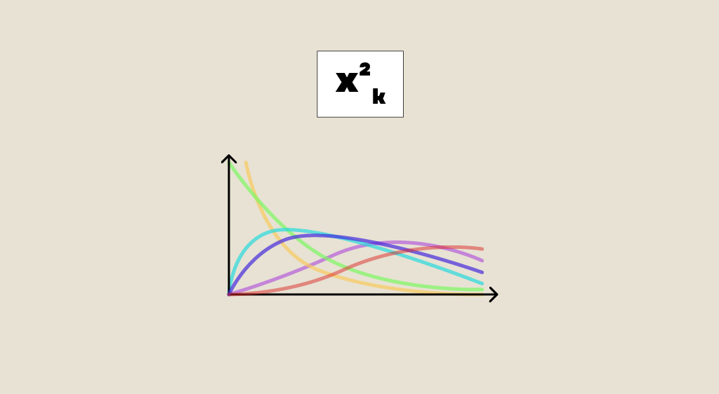
As a reminder, the chi-2 law with d degrees of freedom
centred reduced independent.
is that of a sum of squares of d Gaussians
Otherwise, this statistic will diverge to infinity, reflecting the distance between empirical and theoretical distributions.
Limit formula
What are the benefits of the Chi squared test?
So, we have a simple decision rule: if the Pearson statistic exceeds a certain threshold, we reject the initial hypothesis (the theoretical distribution does not fit the data), otherwise, we accept it.
The advantage of the chi-squared test is that this threshold depends only on the chi-squared distribution and the confidence level alpha, so it is independent of the distribution of the sample.
The test of independence:
Let’s take an example to illustrate this test: we want to determine if the genders of the first two children, X and Y, in a couple are independent?
We have gathered the data in a contingency table:
The Pearson statistic will determine if the empirical measure of the joint distribution (X, Y) is equal to the product of the empirical marginal measures, which characterizes independence:
Here, Observation(x,y) represents the frequency of the value (x, y):
for exemple:
For Theory(x, y), X and Y are assumed to be independent, so the theoretical distribution should be the product of the marginal distributions:
Thus, the theoretical probability for (son, son) is:
Let’s calculate the test statistic using the following Python code:
In our case, the variables X and Y have only 2 possible values: daughters or sons, so the dimension of the problem is (2-1)(2-1), which is 1.
Therefore, we compare the test statistic to the chi-squared quantile with 1 degree of freedom using the chi2.ppf function from scipy.stats.
If the test statistic is lower than the quantile and the p-value is greater than the significance level of 0.05, we cannot reject the null hypothesis with 95% confidence.
Thus, we conclude that the gender of the first two children is independent.
What are its limits?
While the chi squared test is very practical, it does have limitations. It can only detect the existence of correlations but does not measure their strength or causality.
It relies on the approximation of the chi-squared distribution with the Pearson statistic, which is only valid if you have a sufficient amount of data. In practice, the validity condition is as follows:
The Fisher exact test can address this limitation but requires significant computational power. In practice, it is often limited to 2×2 contingency tables.
Statistical tests are crucial in Data Science to assess the relevance of explanatory variables and validate modeling assumptions. You can find more information about the chi-squared test and other statistical tests in our module 104 – Exploratory Statistics.


