In this section, we will focus on one of the most powerful algorithms in Deep Learning: Convolutional Neural Networks (CNNs). These are powerful programming models that enable image recognition, in particular, by automatically assigning a label to each image provided as input, corresponding to the class to which it belongs.
Welcome to the third episode of our Deep Learning series. After introducing Deep Learning and its applications in the first part, and diving into the structure and operation of neural networks in the second, let’s continue our journey!
A convolutional neural network draws inspiration from nature, as the connectivity between artificial neurons resembles the organization of the animal visual cortex.
One of its primary use cases is image recognition. Convolutional networks learn faster and achieve lower error rates in this domain. They are also used, to a lesser extent, for video analysis.
This type of network is employed in natural language processing as well. CNN models are highly effective for semantic analysis, sentence modeling, classification, and translation.
Compared to traditional methods like recurrent neural networks, convolutional neural networks can represent different contextual realities of language without relying on a sequential assumption.
Convolutional networks have also been applied in drug discovery. They aid in identifying potential treatments by predicting interactions between molecules and biological proteins.
CNNs have notably been used in game software for Go and chess, where they can excel. Another application is anomaly detection in input images.
Convolutional Neural Network-CNN architecture
Convolutional Neural Networks (CNNs) constitute a subcategory of neural networks and are currently one of the most renowned models for image classification due to their exceptional performance.
Their mode of operation may seem simple at first glance: the user provides an input image in the form of a pixel matrix. This image has three dimensions:
Two dimensions for a grayscale image. A third dimension with a depth of 3 to represent the fundamental colors (Red, Green, Blue).
Unlike a standard Multi-Layer Perceptron (MLP) model, which contains only a classification part, the architecture of the Convolutional Neural Network has two distinct parts:
1. Convolutional Part: Its ultimate goal is to extract specific features from each image by compressing them to reduce their initial size. In summary, the input image goes through a series of filters, creating new images called convolution maps. Finally, the obtained convolution maps are concatenated into a feature vector called the CNN code.
2. Classification Part: The CNN code obtained as the output of the convolutional part is fed into a second part, consisting of fully connected layers called a Multi-Layer Perceptron (MLP). The role of this part is to combine the features of the CNN code to classify the image. For more information on this part, feel free to refer to the article on the subject.
Convolution part: What is convolution used for?
First of all, what is convolution used for?
Convolution is a simple mathematical operation generally used for image processing and recognition. Its effect on an image is similar to filtering, which works as follows:
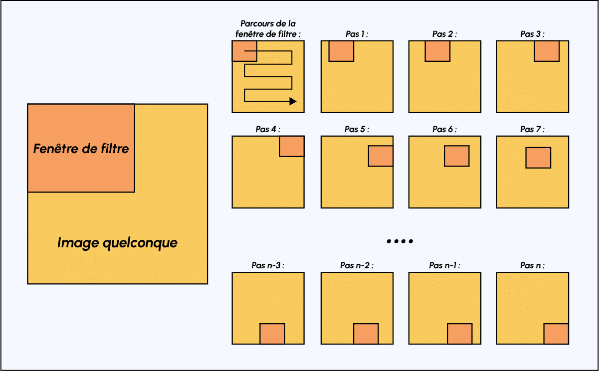
Diagram of how the filter window moves across the image
Initially, you define the size of the filter window, typically starting from the top-left corner.
The filter window, representing a feature, moves progressively from left to right by a predetermined number of cells (the stride) until it reaches the end of the image.
For each encountered portion of the image, a convolution calculation is performed, resulting in an output activation map or feature map that indicates where the features are located in the image. The higher the value in the feature map, the more the scanned portion of the image resembles the feature being sought. This process helps CNNs identify meaningful patterns and features within the input image.
Example of a classical convolution filter
During the convolutional part of a Convolutional Neural Network, the input image passes through a sequence of convolution filters. For example, there are commonly used convolution filters that are designed to extract more meaningful features than individual pixels, such as edge detection (derivative filter) or geometric shape detection. The choice and application of these filters are automatically determined by the model.
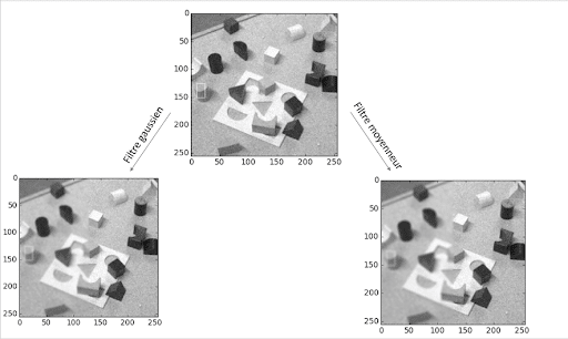
Among the most well-known filters are the averaging filter (which computes the average of each pixel with its 8 neighboring pixels) and the Gaussian filter (which is used to reduce noise in an input image). Here’s an example of the effects of these two different filters on an image with significant noise (imagine a photograph taken in low light conditions, for example). However, one drawback of noise reduction is that it often comes with a reduction in sharpness.
Effect of averaging and Gaussian filters - DataScientest
As you can see, unlike the averaging filter, the Gaussian filter reduces noise without significantly reducing sharpness.
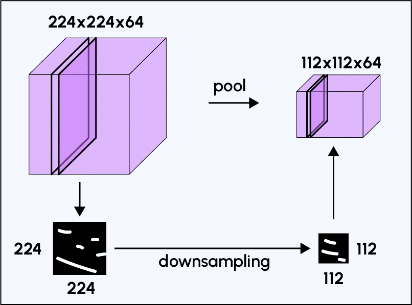
In addition to its filtering function, the convolutional part of a CNN is valuable because it extracts features unique to each image while compressing them to reduce their initial size, using subsampling methods like Max-Pooling.
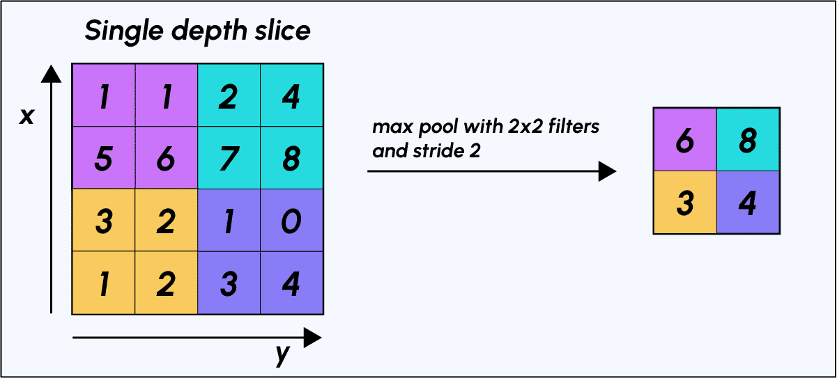
Max-Pooling is a subsampling process based on sampling. Its goal is to downsample an input representation (image, hidden layer output matrix, etc.) by reducing its dimension. Additionally, it reduces computational cost by reducing the number of parameters to learn and provides invariance to small translations (if a small translation does not change the maximum value in the sampled region, the maximum value in each region will remain the same, and therefore, the newly created matrix will remain identical).
To make the action of Max-Pooling more concrete, let’s consider an example: imagine we have a 4×4 matrix representing our initial input and a 2×2 window filter that we apply to our input. For each of the regions scanned by the filter, Max-Pooling takes the maximum value, thus creating a new output matrix where each element corresponds to the maximum value in each encountered region.
Let’s illustrate the process:
Max-Pooling process
The filter window moves two pixels to the right (stride/step = 2) and at each step retrieves the “argmax” corresponding to the largest of the 4 pixel values.
Example of the effect of Max-Pooling
The purpose of the convolutional part of a CNN becomes clearer: unlike a traditional MLP model, adding the convolutional part upstream allows us to obtain an output “feature map” or “CNN code” (the pixel matrix on the right in the example) with smaller dimensions than those of the original image. This significantly reduces the number of parameters to be computed in the model.
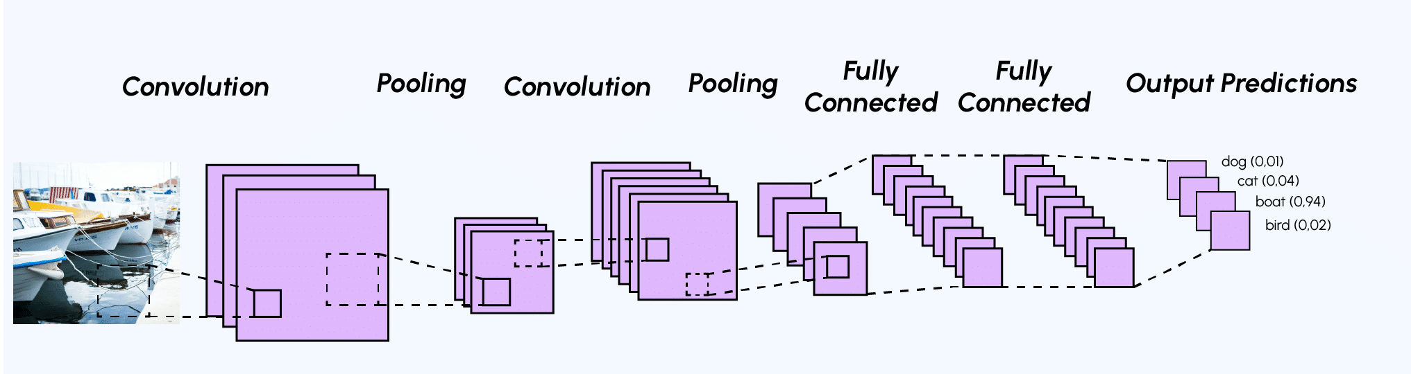
Example of a CNN architecture and its output
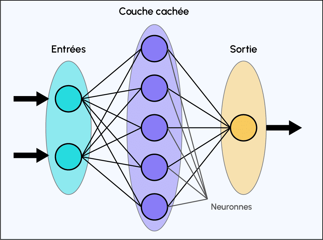
After the convolutional part of a CNN comes the classification part. This classification part, common to all neural network models, corresponds to a Multi-Layer Perceptron (MLP) model.
Its goal is to assign a label describing its class membership to each data sample.
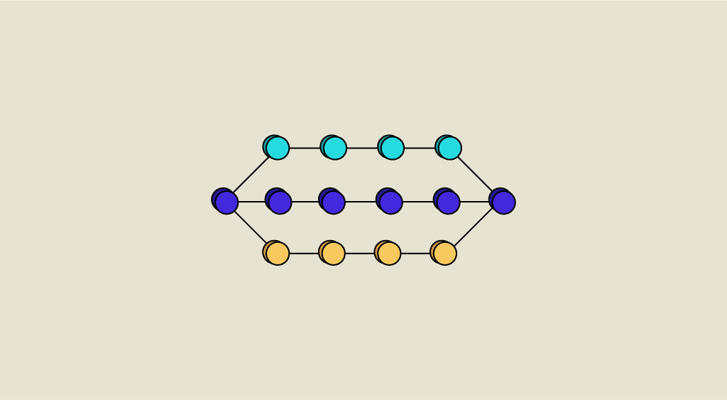
Representation of a multilayer perceptron
The algorithm that perceptrons use to update their weights (or network coefficients) is called backpropagation of the error gradient, a famous gradient descent algorithm that we will delve into in more detail later on.
Example of a CNN architecture
Generally, the architecture of a Convolutional Neural Network is quite similar:
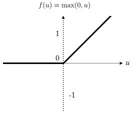
1. Convolutional Layer (CONV): The role of this first layer is to analyze the input images and detect the presence of a set of features. It produces a set of feature maps as output (as explained earlier: what is the purpose of convolution?). 2. Pooling Layer (POOL): The pooling layer is typically applied between two convolutional layers. It takes the feature maps generated by the convolutional layer as input and aims to reduce the size of the images while preserving their essential characteristics. Among the most commonly used pooling methods are max-pooling (mentioned earlier) and average pooling, which calculates the average value of the filter window at each step. 3. Rectified Linear Units (ReLU) Activation Layer: This layer replaces all negative input values with zeros. The purpose of these activation layers is to make the model nonlinear and, therefore, more complex.
The final output of the pooling layer retains the same number of feature maps as input but in a considerably compressed form.
ReLU activation function
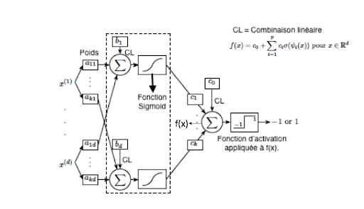
Fully Connected (FC) Layer: These layers are placed at the end of the CNN architecture and are fully connected to all output neurons (hence the term fully-connected). After receiving an input vector, the FC layer applies a linear combination followed by an activation function, ultimately aiming to classify the input image (see the following diagram). In the end, it outputs a vector of size d, corresponding to the number of classes, where each component represents the probability of the input image belonging to a class.
Operation of a neural network with 2 hidden layers
Implementation of a pre-trained CNN on Python :
For practical purposes and given the complexity of creating effective CNNs from scratch, we will use pre-trained networks available in the Torchvision module. Let’s see how this can be implemented in Python:
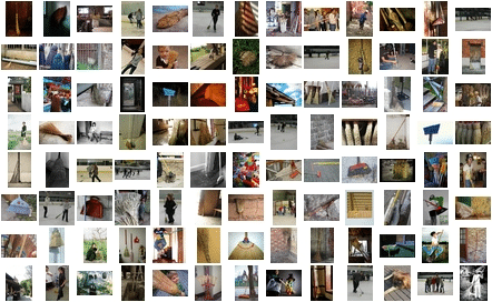
Application of a CNN: Identification of any images from the ImageNet dataset: ten million labelled images
ImageNet is a database of over ten million labeled images produced by the organization of the same name, intended for computer vision research. Here is an excerpt from this extensive dataset:
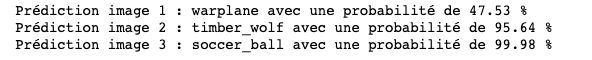
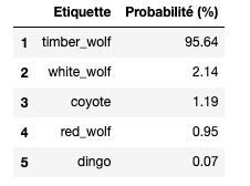
We can also display the 5 labels considered most likely by VGG16 :
Top 5 labels considered most likely by VGG16
→ VGG16 has successfully predicted with high confidence (95.6%) that not only the input image was a wolf but even went further by specifying its breed, which in this case is an Eastern Gray Wolf (timber wolf). Impressive, isn’t it?
In the end, the operating principle of a CNN is quite easy to understand. However, paradoxically, implementing such a process to classify images remains very complex due to the considerable number of parameters to define: the number, size, movement of filters, choice of pooling method, the number of layers of neurons, the number of neurons per layer, and so on.
To overcome this obstacle, Python, through the Torchvision module, offers the possibility to use powerful pre-trained CNN models such as VGG16, Resnet101, etc.
In this article, we’ve explained the operation and architecture of Convolutional Neural Networks, with a focus on its specificity: the convolutional part.
We still have one more step in classification to cover: backpropagation of the error gradient, the famous gradient descent algorithm. Don’t worry, the next episode on this topic will be coming soon on the blog!
Facebook
Twitter
LinkedIn
DataScientest News
Sign up for our Newsletter to receive our guides, tutorials, events, and the latest news directly in your inbox.
You are not available?
Leave us your e-mail, so that we can send you your new articles when they are published!