
Large data sets can be easily analyzed and organized using Microsoft Excel. But it is very useful to know How to freeze rows in Excel...
However, when working with large spreadsheets, it’s easy to lose track of what each column or row represents. For data analysis, good visibility is essential. But when spreadsheets comprise several hundred rows, it’s easy to lose your bearings. That’s why it’s best to freeze a row in Excel. We’ll show you how to freeze rows in Excel.
Why freeze rows in Excel?
While Excel spreadsheets are invaluable analysis tools, they sometimes include several hundred or even several thousand lines of data. Such a large amount of information makes processing more complex. When you scroll down the spreadsheet, you won’t always know which category a particular cell belongs to. In this case, you often have to go all the way back to the first line. This is a real waste of time, especially if you have several hundred rows to analyze.
Fortunately, it is possible to freeze a line in Excel to keep the most important cells (usually the header).
For example, for a customer prospecting file, you can freeze the first few lines. These specify the various categories, such as prospect/customer name, contact details, personal situation, maturity level, etc. This way, when you scroll down your spreadsheet, you’ll always know what each cell corresponds to.
With this method, when you know how to freeze rows in Excel, you save time and improve your productivity.
How to freeze rows in Excel ?
If you want to keep your spreadsheet header, simply freeze the first line. It’s very simple:
Select a table cell (any cell);
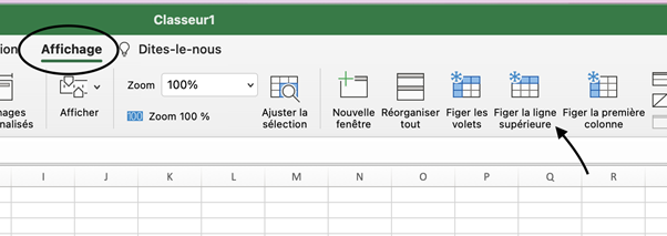
Click on “View”, “Freeze panes”, then “Freeze top row”.
The first line remains fixed. This allows you to scroll your Excel spreadsheet downwards, while retaining visibility of the various categories.
You can repeat the same operation if you wish to freeze a column in Excel. In this case, simply select “Freeze first column”.
This locks the first line of your spreadsheet, ensuring that it remains visible when you browse the rest of the sheet.
How do I freeze several lines in Excel?
Beyond the first line, it’s also possible to freeze several lines in Excel. Here’s how to do it:
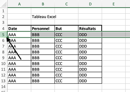
Select the first cell not to be frozen. For example, if you wish to freeze the first three rows, select cell C1 ;
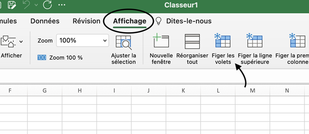
Click on “View”, then “Freeze panes”.
You will then be able to scroll down the spreadsheet, while retaining visibility of the first three rows.
Once again, the same procedure can be used to freeze columns. For example, if you wish to freeze the first three columns, select cell A4.
Select “View” from the drop-down menu, then “Freeze panes”.
When many rows are frozen, they always remain at the top of the document when scrolling.
Only rows at the top of the sheet can be frozen.
If you wish to “freeze” rows in the center of the page, this will be impossible from a practical point of view.
Be sure to keep lines visible before freezing them. After freezing, invisible lines will be hidden and inaccessible.
Is it possible to freeze rows?
In addition to freezing Excel rows (or columns), you can also freeze rows and columns at the same time. To do this, follow these steps:
Select the first cell not to be frozen. For example, if you wish to freeze the first three rows and two columns, select cell C4 ;
Click on “View”, then “Freeze panes”.
Here, your columns and rows are frozen.
How do I undo a row or column freeze in Excel?
While it’s very easy to freeze a line in Excel, it’s also very easy to make a mistake when doing so. In other words, you may have frozen lines that are not relevant to your analysis. In this case, you’ll need to defreeze these lines.
Once again, it’s very simple. Here’s how it works:
Click on the “freeze row” button to bring up additional options, then click on defreeze to release the panes.
From now on, your Excel table is completely free. You can leave it as it is, or freeze the rows or columns you need (without making a mistake this time).
What other solutions are there for freezing rows or columns in Excel?
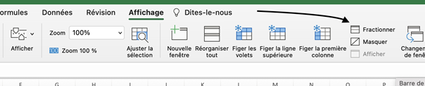
Use the “Split” function if the “Freeze shutters” option doesn’t suit you or simply doesn’t work. It’s right next to the block above.
Unlike the “Freeze panes” tool, this tool divides an Excel document into several pieces rather than freezing the rows. They become independent of each other and can be scrolled separately.
Let’s put this separation to the test:
Select the cell below the lines you wish to split. Then select “Split”.
A separation bar appears above the selected cell. As you scroll down the page, you’ll notice that the rows remain in place.
To cancel the split, simply click on the “Split” item again, and the sheets will become a single whole again, without any further row splitting.
You now know how to freeze the first two rows of Excel, or many rows of a worksheet. We hope you find this Excel tutorial useful!
💡Related Articles:
Things to remember
- Freezing a row in Excel gives you a clear view of the different categories in the table.
- You can freeze one row, one column, several rows, several columns, or both.
- If you make a mistake, you can also easily undo a line in Excel.


