One of the most effective ways of representing data in a clear and comprehensible way is to create diagrams and charts. Microsoft Excel offers users a wide range of analysis options. It is therefore possible to gain greater visibility over your numerical data by creating charts in Excel.
In presentations, charts and graphs are often used to provide a quick overview of a trend in results, or to highlight the distribution of a set of data according to certain variables. You can create a table or graph to represent almost any type of quantitative data, so you don’t have to sift through spreadsheets to discover relationships and trends.
Follow these simple steps and learn how to create your own Excel chart:
Please note! If you have created an Excel chart from this data and add new data to your table, the new data will not be automatically updated in the chart. In order to take them into account, you’ll need to create a new chart, selecting the new integrated data.
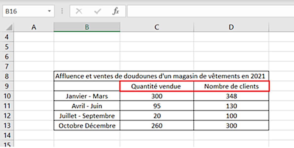
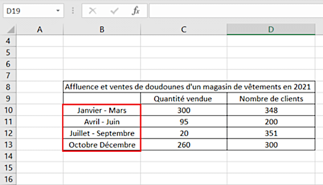
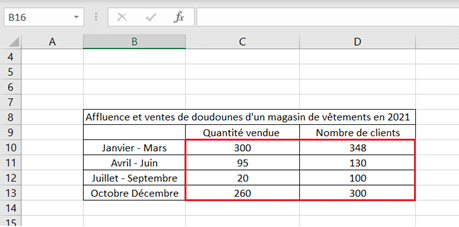
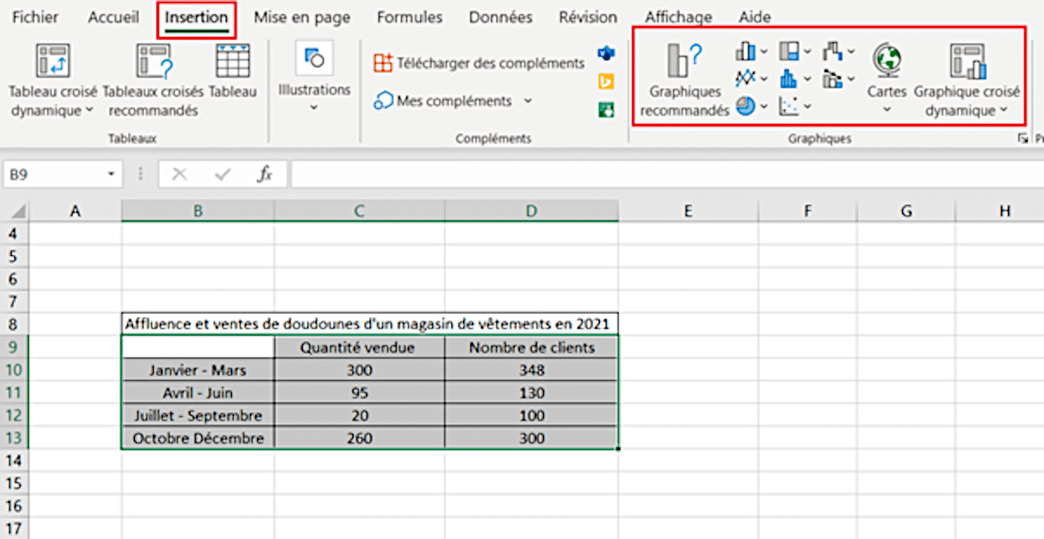
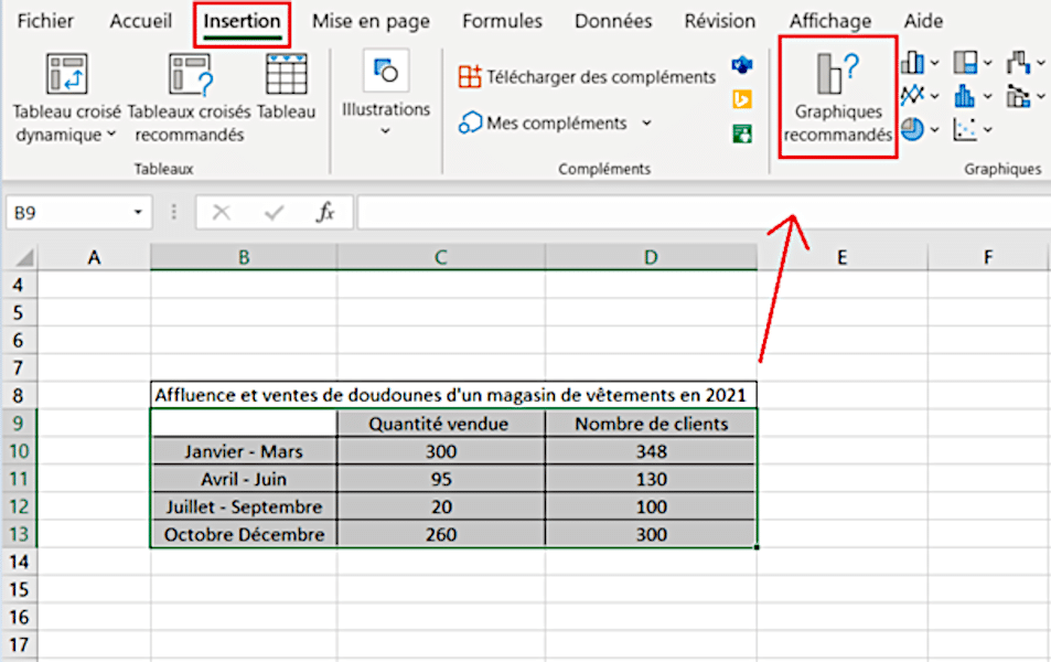
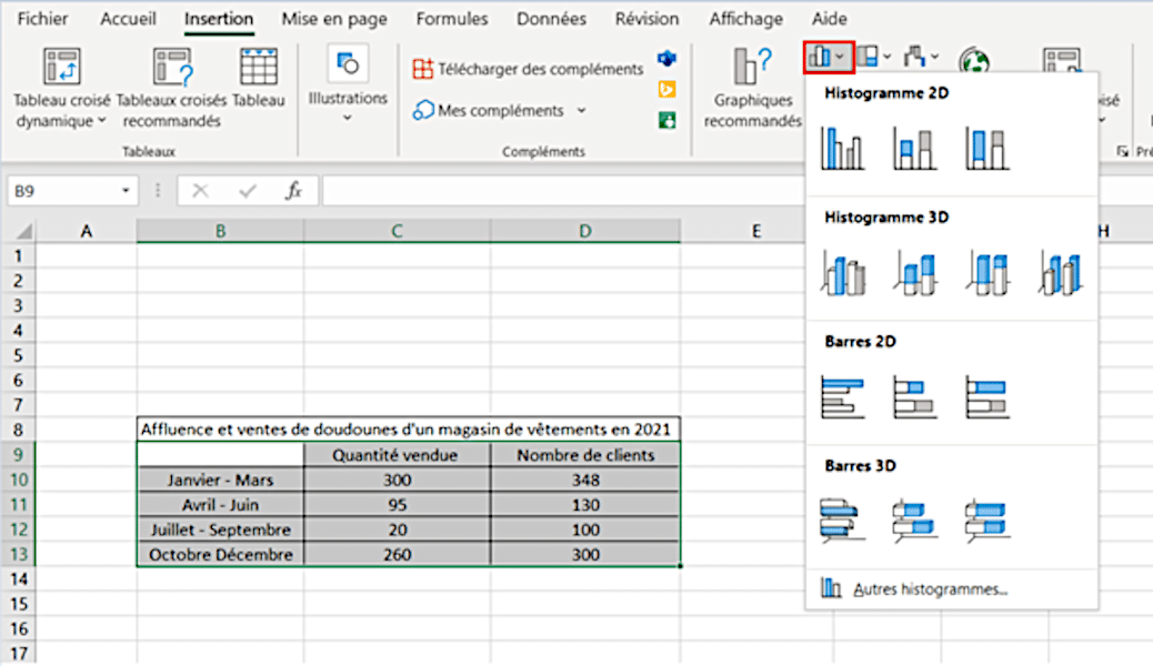
5. Select your data, then click on the Insert tab to select the chart of your choice. It’s important to select the right data, headers and labels to ensure that your chart is complete and, above all, legible.
In Excel, you can create different types of chart, each ideal for different types of data.
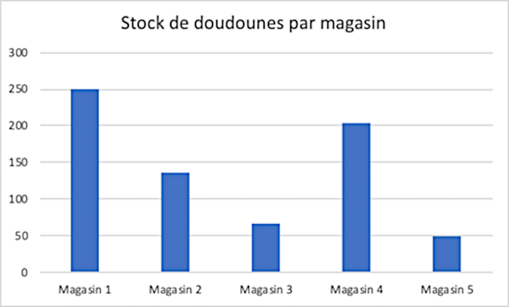
Vertical charts are used to display one or more data sets, and are ideal for comparing two similar data sets, or for listing data differences over time.
For example, a vertical chart can be used to represent the stock of down jackets in different stores of the same brand.
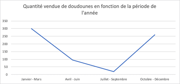
Line graphs use horizontal lines to display one or more sets of data. Ideal for displaying the increase or decrease of data over time.
For example, these graphs are highly relevant for analyzing a company’s sales evolution, to give visibility on the different trends that may exist over a sales year.
For example, a graph of this type can be used to model the number of down jacket sales according to the time of year.
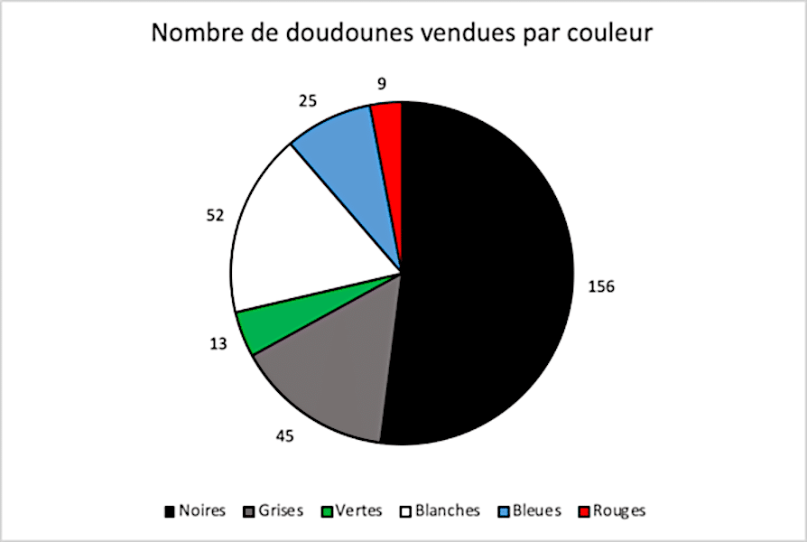
Pie charts show a single set of data as fractions of a whole. Ideal for visually displaying the dispersion of data. For example, if you want to display the percentage of down jackets sold by down jacket color:
Excel’s “Recommended Charts” function can help you select the appropriate type of chart or diagram.
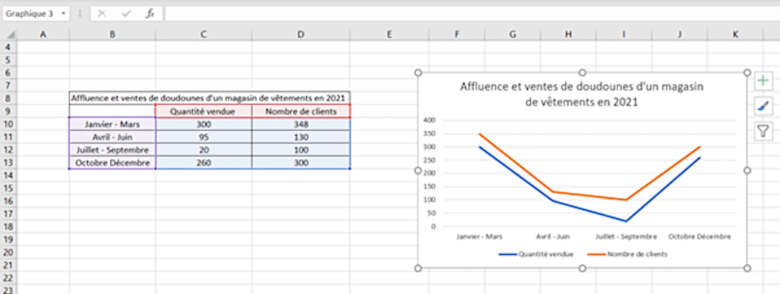
Using the data entered, here is the graph obtained:
In this example, the aim is to analyze the evolution of sales as a function of time, taking into account the store’s affluence and the time of year. A line graph makes it easy to identify correlations between variables. For example, we can see that the sale of down jackets is highly dependent on the number of customers and the season. The variables “Quantity sold” and “Number of customers” are said to be correlated; the curves have the same shape.
7. Choose a format for your graph in Excel. Select a suitable version of the chart from the drop-down menu of the selected chart. Modify the format and style of your chart.
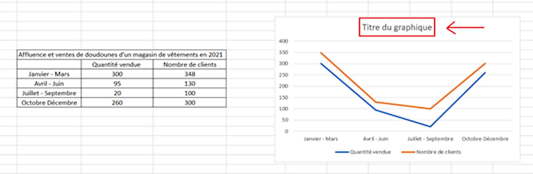
8. Add a title to your graph. Double-click on the “Chart title” text at the top of the chart, then replace the text with your own title. If necessary, rearrange your data.
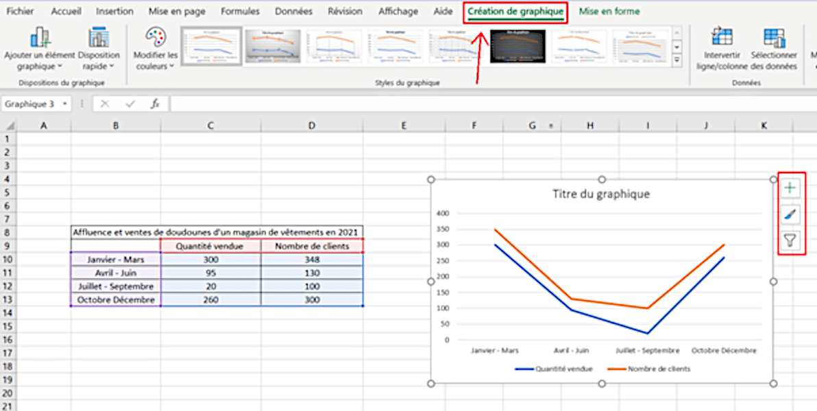
9. Customize your chart.
Select your chart and click on the Chart creation option in the main menu at the top of the screen to access the main modifications.
Customization options are also available by clicking on the small boxes to the right of the chart. You can, for example, swap chart columns or filter the data to be displayed.
10. Save your graph. To do this, click on File, Save as, double-click on “This PC”, select a location to save the file, give the document a name in the “File name” text box and save.
Use a keyboard shortcut to quickly create your Excel chart
There’s a keyboard shortcut for quickly creating a chart: Alt+F1.
To do this, first select the data in your table, then apply the shortcut. Excel will generate a chart template based on the data you’ve chosen. You can always modify it if you don’t like it.
Want to take your Excel skills to the next level? DataScientest offers Excel training courses from 3 to 6 days, 100% financed by the Compte Formation. Our training courses enable you to master the various Excel functions up to Expert level, and prepare you to take the official TOSA exam.