In this article, we present one of the pitfalls of supervised learning algorithms: overfitting.
What is overfitting?
Overfitting in Machine Learning is the risk of a model learning the training data “by heart”. In this way, it runs the risk of not being able to generalize to unknown data.
For example, a model that returns the label for training data and a random variable for unknown data would perform very well during training, but not for new data.
When is overfitting likely to occur?
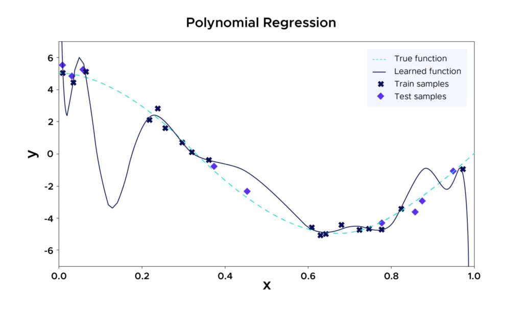
Overfitting occurs when the chosen model is too complex relative to the size of the dataset. For example, in the case of a polynomial regression with a high degree, the model tries to fit to a large number of training points, which can result in neglecting many other unseen points. Although this machine learning model may perform excellently on the training data, it runs the risk of producing a huge squared error on unseen data.
Why is overfitting a problem?
Overfitting can lead a model to poorly represent the data on which it was trained. As a result, its accuracy will be lower on new, similar data compared to an ideally fitted model. However, when applied to the training data, the overfitted model may appear to offer higher accuracy. It’s therefore easy to be misled.
Without protection against overfitting, developers can train and deploy a model that appears highly accurate at first glance. In reality, this model will perform poorly in production on new data.
Deploying such a model can cause various problems. For example, a model used to predict the likelihood of a payment default may announce a much higher percentage than reality in the case of overfitting. This can lead to poor decisions, resulting in financial losses and customer dissatisfaction.
Overfitting vs Underfitting
In contrast to overfitting, underfitting occurs when training data is highly biased. For example, if a problem is overly simplified, the model will not perform correctly on the training data.
It can be caused by data containing noise or erroneous values. The model will therefore be unable to identify patterns from the dataset.
Another cause can be a highly biased model due to its inability to capture the relationship between training examples and target values. The third reason can be a model that is too simple, such as a linear model trained on complex scenarios.
In an attempt to avoid overfitting, there is a risk of causing underfitting. This can happen by interrupting the training process too early or by reducing its complexity by removing less relevant inputs.
If training is stopped too early or important features are removed, underfitting can occur. In both cases, the model will be unable to identify trends within the dataset.
Therefore, it is essential to find the ideal balance where the model identifies patterns in the training data without memorizing overly specific details. This will allow the model to generalize and make accurate predictions on other data samples.
How to avoid overfitting?
To avoid overfitting, it is essential to evaluate the model on unseen data each time.
A good practice is to split your initial dataset into a training set and a test set. The training set is used to train the model, while the test set, consisting of unseen data, is used to assess how well the model generalizes.
One can only draw conclusions about the model’s performance based on the test set’s performance, not on the training set’s performance, which may be memorized by the model.
How to avoid overfitting? How to select training and test data?
The simplest and most commonly used method is to randomly split the data. The Python sklearn.model_selection module provides the train_test_split function for this purpose. By providing it with a dataset, this function creates a partition of the data, allowing you to obtain the test set and the training set.
However, this random splitting comes with a risk of creating unrepresentative datasets by chance.
To avoid validating a model on unrepresentative data, one method is to replicate the training and testing procedure multiple times on different splits and then average the results. This helps smooth out the random effects and provides an estimate of the model’s performance on randomly chosen unseen data.
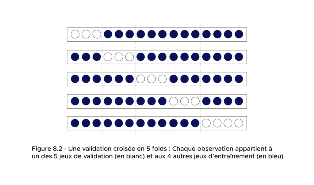
This model validation technique is called cross-validation.
Cross-validation is composed of multiple folds. Each fold involves partitioning the dataset into two sets: a training set and a test set. For each fold, the model is trained on the training set and evaluated on the test set.
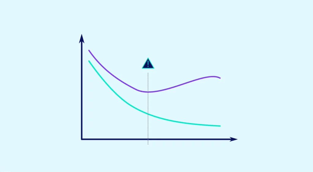
The performance of the model is then estimated by evaluating the performance of the predictors from each fold on the test set of each of the other folds and averaging their performances.
This approach also allows access to the standard deviation of these performances, providing insight into the variability of the model’s performance depending on the training set. If the variability is high, then it’s crucial to be cautious about the choice of the training set. Conversely, with low variability, the choice of the training set has less impact.
What are the sources of error in a model?
For a regression model, the primary evaluation criterion is the Mean Squared Error (MSE).
Let’s break down the Mean Squared Error (MSE) on a dataset D for an estimator into the following components:
1. The square of the bias of the estimator (which quantifies how far the predicted labels are from reality).
2. The variance of the estimator (which quantifies how much the labels vary for the same individual based on the input data).
3. The variance of the noise, also known as irreducible error.
Therefore, a biased estimator with low variance can sometimes achieve better performance than an unbiased estimator with high variance.
In many cases, overfitting occurs when choosing an unbiased estimator with high variance. Complex models can exhibit these characteristics, such as high-order polynomial regressions (see diagram 1). Opting for simpler models that are inherently “less good” due to bias can lead to better performance if their variance is low.


