New appointment with Daniel, the technical support for DataScientest. the data science expert who accompanies learners throughout their training courses. Today, he talks to us about time series. Time series is one of the most widely studied topics in data science. In this article, you'll discover the main components of a time series.
What is a time series?
Time series cover a wide range of real-life phenomena and can be found in many fields.
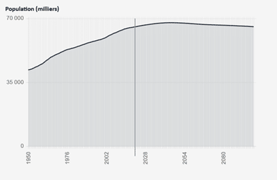
A time series can be anything from the evolution of a country’s population or GDP, to an electrocardiogram or the latest Dua Lipa soundtrack.
Mathematically, a time series is a series of data indexed by time.
The analysis and prediction of these series is therefore of prime interest to certain industries or sectors, because in practice, predicting a time series means predicting the future.

How do you break down a time series?
Traditionally, a time series is broken down into three elements:
- A trend (Tt)
- Seasonality (St)
- A residual or error (εt)
Mathematically, a time series can be expressed as Xt = Tt + St + εt
With T the trend, S the seasonality, ε the residual and t the time index.
The trend
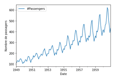
A trend is the increasing or decreasing behavior of a series over time. It often reflects a phenomenon of growth or decline over the long term.
The trend of a time series can take different forms:
- Linear Tt = α + βt
- Quadratic Tt = α + βt + γt²
- Exponential Tt = α + βexp(t)
….
Seasonality
Seasonality reflects the presence of a periodic phenomenon that repeats itself throughout the time series.
Thus, if the seasonal component repeats itself according to period k. St+k = St
Seasonality is a feature of many data, particularly meteorological data (temperature changes over time).
Some time series show both a trend and a seasonal pattern, as in the case of global air traffic. Air traffic is on the rise, but there is a marked difference between winter and summer traffic.

The residue
The model residual is the part of the time series that cannot be explained by decomposition. A time series cannot be completely decomposed according to trend and seasonality alone.
Ideally, the residual of the model is stationary, i.e. the remaining process does not evolve over time (constant mean and variance). If the residual of our time series is not stationary, this means that certain temporal components are not explained in the model.
Once the trend and seasonality of the time series have been explained, we can then try to explain the decomposition residual using auto-regression or moving-average processes, which gave rise to the famous ARMA model.
The holy grail of time series modeling is to obtain a white noise residual, i.e. one that no longer contains any temporal information. In practice, this means a random, decorrelated stationary signal.
Further information
– In addition to seasonality, we sometimes define a cycle that can be considered as a longer-period seasonality, in which case we can define several different cycles.
– The presence of seasonality between two dates can make comparison between these dates difficult. Depending on the problem, we may therefore seek to correct for seasonal variations in time series. This is the case, for example, with the unemployment rate or growth rate.
– The decomposition Xt = Tt + St + εt is said to be additive, but we can also model a time series according to a multiplicative decomposition Xt = Tt (1 + St )(1 + εt )
Conclusion
In this article, you’ve learned about the basics of time series: trend, seasonality, residual, white noise and stationarity.
However, beyond time series, data science covers many other issues (computer vision, natural language processing, data vizualization, etc.) which we invite you to discover by following one of our Data Scientist or Data Engineer training courses.


