The performance of a Machine Learning algorithm is directly related to its ability to predict an outcome. When comparing the results of an algorithm to reality, a confusion matrix is used. In this article, you will learn how to read this matrix to interpret the results of a classification algorithm.
What is a confusion matrix?
Machine Learning involves feeding an algorithm with data so that it can learn to perform a specific task on its own. In classification problems, it predicts outcomes that need to be compared to the ground truth to measure its performance. The confusion matrix, also known as a contingency table, is commonly used for this purpose.
It not only highlights correct and incorrect predictions but also provides insights into the types of errors made. To calculate a confusion matrix, you need a test dataset and a validation dataset containing the actual result values.
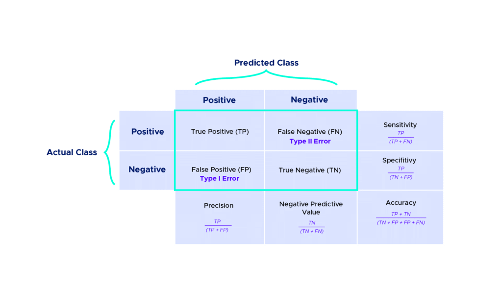
Each column of the table represents a class predicted by the algorithm, and the rows represent the actual classes.
Results are classified into four categories:
True Positive (TP): The prediction and the actual value are both positive. Example: A sick person predicted as sick.
True Negative (TN): The prediction and the actual value are both negative. Example: A healthy person predicted as healthy.
False Positive (FP): The prediction is positive, but the actual value is negative. Example: A healthy person predicted as sick.
False Negative (FN): The prediction is negative, but the actual value is positive. Example: A sick person predicted as healthy.
Of course, in more complex scenarios, you can add rows and columns to this matrix.
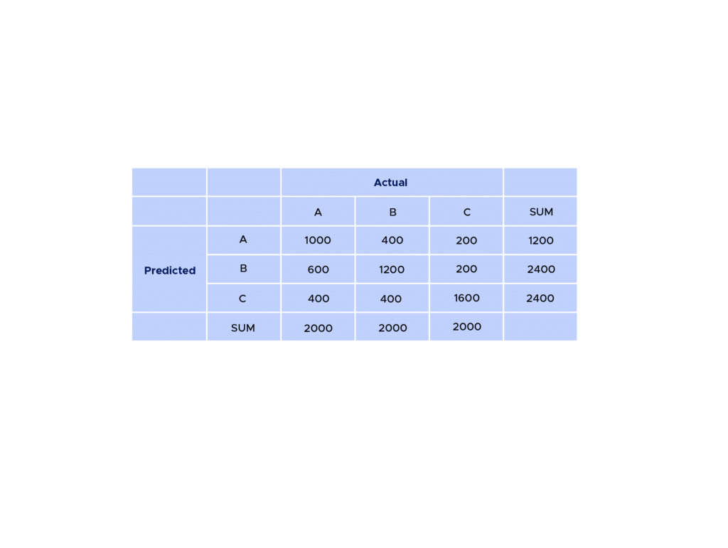
Example: After applying a predictive model, we obtain the following results:
In general, you always find the correct predictions on the diagonal. So, here we have:
– 600 individuals classified as belonging to class A out of a total of 2000 individuals, which is quite low. – For individuals in class B, 1200 out of 2000 were correctly identified as belonging to this class. – For individuals in class C, 1600 out of 2000 were correctly identified.
The number of True Positives (TP) is therefore 3400.
To calculate the number of False Positives (FP), True Negatives (TN), and False Negatives (FN), it’s not possible to calculate them directly from this table. You would need to break it down into three cases:
1. Individuals in A and not in (B or C) 2. Individuals in B and not in (A or C) 3. Individuals in C and not in (A or B)
You can then calculate all the necessary metrics for analyzing this table.
Here are some common metrics derived from this kind of table:
Quelles mesures devrions-nous utiliser pour évaluer nos prédictions ?
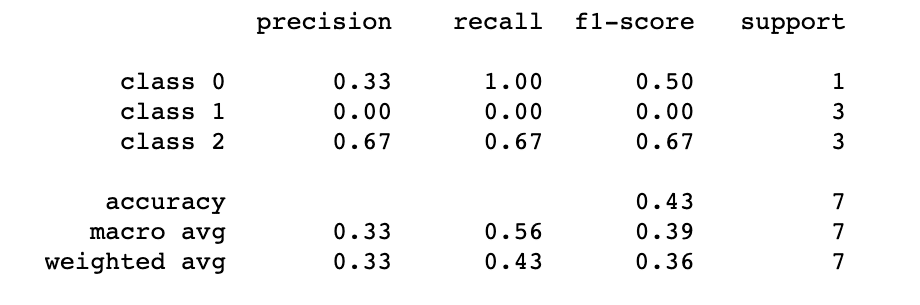
Here, we chose to name the different classes based on the values of y_true. We can then observe various metrics that allow us to assess the quality of our predictions, primarily:
These metrics provide valuable insights into the performance of a classification model. Precision measures the accuracy of positive predictions, recall measures the ability to correctly identify positive cases, and the F1-score is a balanced measure that combines both precision and recall into a single value.
In our case, we can observe a Precision of 0 for class 1. This is simply because no individuals from real class 1 are predicted as belonging to that class. In contrast, for individuals in class 2, where 2 out of 3 were correctly assigned to class 2, we have a Precision of 0.67.
Precision measures how many of the predicted positive cases were correct, so when there are no positive predictions for a particular class, the Precision for that class becomes 0. It’s an important metric for understanding the model’s ability to avoid false positives for a specific class.
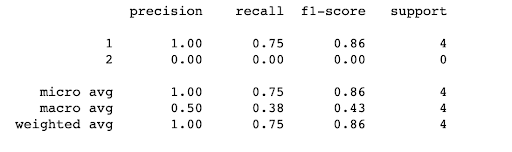
The differences between micro-betterment and macro-betterment
The calculation and interpretation of these averages are slightly different.
Regardless of the metric used, a macro-average calculates an average after calculating the metric independently for each class. In contrast, a micro-average takes into account the contributions of each class to calculate the average metric.
In a multi-class classification, this approach is often favored when there is suspicion of imbalance between the classes (in terms of sample size or importance).
For example:
This gives us the following result:
You now know how to read and interpret the results of a classification algorithm. If you want to learn more about this topic, you can check out our Data Analyst, Data Scientist, and Data Manager training programs, which cover these concepts in more practical cases.