Welcome to the second part of this dossier dedicated to Vector Machine Support.
In the previous article, we detailed the operation and main shortcomings of Maximal Margin Classifiers.
Our aim now is to allow our algorithm to make a certain number of errors when selecting the separation line. This is known as the “soft margin”. We will now describe in detail how the Soft Margin Classifiers algorithm works, halfway between the Support Vector Machine and the Maximal Margin Classifier.
Soft Margin Classifiers
In the previous article, we defined the margin as the distance separating a line from the nearest observation.
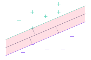
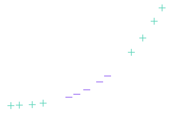
In this second part, we’ll also use the term margin, but this time it will refer to the set of points closer to the line than the nearest observation
Here, for example, the margin is the area shown in pink on the graph. In fact, it’s the space between the 2 outer lines.
To make our algorithm more flexible, we’ll use a threshold, which corresponds to the number of observations we’ll tolerate within the margin.
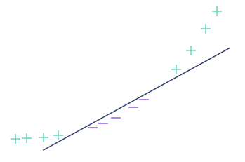
Then, as before, we’ll try to determine the dividing line that maximizes the margin.
However, we are no longer concerned with the observations inside the margin. This allows us to achieve a certain insensitivity to extreme values.
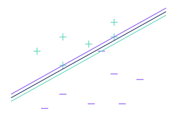
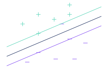
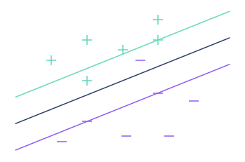
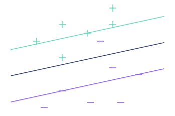
Here’s what we get in the previous example with different threshold values:
In reality, when you increase the threshold, you decrease the variance but increase the bias. In jargon, the higher the threshold, the lower the risk of overfitting.
⚠️Note: Observations within and at the boundaries of the margin are called Support Vectors, and the Soft Margin Classifiers algorithm is also called Support Vectors Classifier.
Support Vector Machine
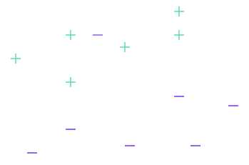
We have found a solution to the first problem, but not to the second. The Support Vector Classifier algorithm still doesn’t work in the following case:
In fact, when the algorithm doesn’t work, the data is said to be non-linearly separable, and there are mathematical tools for determining whether a dataset is, or is not, linearly separable.
When faced with a dataset, we use these tools. If the dataset is linearly separable, you don’t need to look very far – just apply the Soft Margin Classifier. Things get trickier, however, when the dataset is not linearly separable.
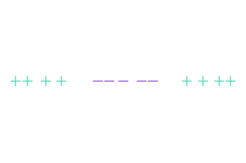
To simplify visualization, we’re going to change the dataset, and this time take observations of dimension 1, i.e. on a straight line (and not a plane).
There’s no need to explain why no straight line can separate the “+” and “-” in this particular configuration.
The idea of the Support Vector Machine is to project the data into a higher-dimensional space, to make it separable.
Returning to our 1-dimensional example, we’re going to project the data into a 2-dimensional space. To do this, we’ll need what we call a kernel function. The kernel function acts as an intermediary between the two spaces.
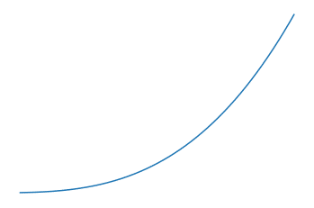
Let’s take the cube function (f(x) = x^3) as an example. Here’s how to apply the kernel function to the dataset to project it into a 2-dimensional space:
In other words, if we denote f the kernel function, for each observation x, we place a point with coordinates (x, f(x)) in the plane.
The projected dataset is now separable, as shown in the following image. The Soft Margin Classifiers algorithm described above can be used to calculate the best separation line, and that’s all there is to it.
We’ve just described in detail how Support Vector Machines work. And even though we’ve deliberately left out some of the details (such as the choice of kernel function), you now have an overview of the subject.
SVM algorithms can be adapted to classification problems involving more than 2 classes, and to regression problems. They are therefore quick and easy to implement on any type of dataset, which certainly explains their success.
Where a neural network requires upstream work to determine the right structure and parameters to use, SVMs achieve good results even without preparation. If you’d like to learn more about Machine Learning, take a look at our Machine Learning Course.