Welcome to the first part of this mini-series dedicated to SVM.
When we think of Machine Learning, we generally think of recent methods that are still poorly understood and used empirically, like a sorcerer’s apprentice.
Indeed, genetic algorithms, neural networks, boosting… these algorithms are often described as “black boxes”. In other words, while it’s easy to comment on the input and output of the algorithm independently, when it comes to detailing the exact contribution of each input to the final result, it’s a different kettle of fish. Blame it on too many parameters, the use of random events…
Nevertheless, among this myriad of algorithms, each more complex than the last, there is one whose advanced age belies its effectiveness and simplicity.
Conceptualized by Vladimir Vapnik in the early 60s, it entered the computer world in 1990. Since then, it has become a reference for all those interested in supervised learning techniques. Even today, it continues to be taught, studied and widely used. As you may have gathered, we’re talking about Support Vector Machines (SVM).
⚠️Warning: talking about the simplicity of such an algorithm is like talking about the smallness of the Moon. We know it’s small compared with its surroundings, but we couldn’t possibly walk around it.
This article will be divided into 2 parts. In the first, we’ll introduce you to the basic principle of Margin Classifiers, and their limitations.
In the second part, we’ll go into more detail about SVMs, with the aim of providing an overview of how they work.
Maximal Margin Classifiers
As is often the case in science, before tackling the problem as such, we prefer to study a particular case, which is simpler to solve. So we’ll begin this presentation with a study of a cousin of SVMs, Maximal Margin Classifiers.
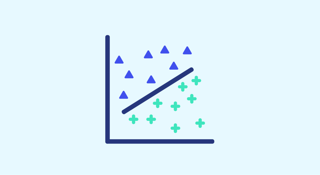
Suppose we have a dataset containing 2 types of observations: “+” and “-“. Our objective is to be able to predict the class (“+” or “-“) of a new observation, represented here by an “x”.

Instinctively, we understand that the observation should be classified as a “-” here. But it’s difficult to explain the reasons why.
We’ll apply the following method:
Draw a straight line separating the 2 classes. If the observation lies above this line, we’ll call it a “+”, otherwise a “-“. Here, for example, observation “x” is above the line, so it’s a “-“.
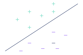
The method seems to work well. However, in the particular case of our problem, there are an infinite number of straight lines perfectly separating the 2 sets.
Each of them delimits a different space and represents a different answer to the problem. The question is how to choose the best straight line from all the possible ones.
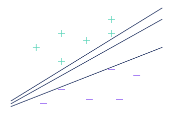
On the previous figure, it seems logical to say that the central line separates the data better than the other 2. Indeed, as it is far from both the “+” and the “-“, it is unlikely to classify an observation in one class when it is actually very close to the other.
In mathematics, the distance separating a straight line from the nearest observation is called the margin. The central straight line has a larger margin than the other two.
In other words, the straight line that best separates the 2 classes is the one with the highest margin. Do you now understand where the term “Maximal Margin Classifiers” comes from?
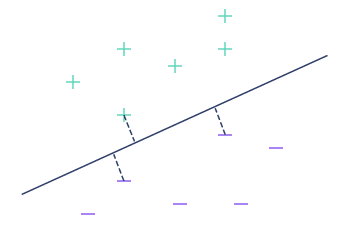
In our example, the continuous line is the best separating line. The margin, shown as a dotted line, is maximum. You’ll have noticed that the same distance separates the straight line from the 3 nearest observations. This is a characteristic that is systematically found for the best straight line.
The Maximal Margin Classifier algorithm uses this method to calculate the best straight line.
What’s important to remember from this introduction is that it’s enough to find the line with the largest margin to be able to classify all new observations.
What’s more, when it exists, it’s relatively simple to calculate the equation of the separation line (if you’re interested in the details of the calculations, I recommend the MIT OpenCourseWare video, which deals precisely with this subject .
This is a quick and easy way to answer the problem at hand.
However, the method we’ve just seen has two major shortcomings. It is highly sensitive to extreme values (also known as outliers).
The arrival of an outlier (the highest “-“) completely disrupts the result.
Worse still, in case you were wondering: No, there isn’t always a straight line separating the 2 classes perfectly. This is the case, for example, in the following image:
In the end, we end up with an algorithm that, in some cases, doesn’t work at all.
In the next article dedicated to SVMs, we’ll look at how we can give our algorithm more flexibility, by allowing it to make a few classification errors, to improve its overall performance.
Are you interested in Machine Learning techniques? Would you like to learn how to master them? Our data science training courses are just what you need!


