It's highly likely that you use applications that make use of Deep Learning models in your day-to-day work. Translation, ocr, facial recognition... Many of your applications incorporate deep learning.
This application of Deep Learning has been made possible by the availability of the large quantities of data that algorithms need to be effective, and by advances in machine computing power that enable these algorithms to be trained.
It is possible to build Deep Learning models and train them in several languages, but in this article we will use Python and its libraries designed specifically for Deep Learning: Tensorflow and Keras.
Keras is an open source library designed to provide all the essential tools for experimenting with neural networks. You need to have the library installed on your work environment.
The Google Colab environment provides the essential prerequisites for Deep Learning and Data Science.
Train your first neural network
Now that you’ve learned about the tools you need to use to perform Deep Learning, it’s time to get your hands dirty and build, train and evaluate your first Deep Learning model.
But you won’t be alone: we’ve put together a tutorial covering the main steps a data scientist takes to train a neural network.
We’ll explain these steps so that you can carry out the process for your future modelling.
First, open your Jupyter or Colab notebook to tackle the first step. You can simply copy the cells to your Notebook, but we strongly advise you to code them yourself so that you can understand the syntax better. Remember, practice makes perfect.
Loading data :
It’s well known that to carry out a Deep Learning project (or to do Data Science in general), you need a large quantity of data. So the first step is naturally to select and import our data.
The dataset we’re going to use is very familiar to data scientists: it’s the MNIST dataset, which contains almost 60,000 28×28 pixel images of handwritten numbers with numeric numbers as the target variable. The objective of our model will be to recognise the number written on the image.
You will find on the script the import of the libraries needed for our modelling. You will also notice that the dataset is included in the Keras module and that we have two different sets of data, the training part (train) and the test part (test).
The result of executing this first cell will be the size of the dataset and the dimensions of the images.
Here we’re going to take a look at a random sample of images with their corresponding labels.
Here’s an example of how to execute the above cell.
Data pre-processing
Once your data has been loaded, you need to ensure that it is ready for the training phase. To do this, you will apply a number of transformations to the data. These include resizing, normalising and encoding the data.
But don’t panic, once again we’ll walk you through the process and each pre-processing step will be explained.
Resizing: One of the special features of machine learning and deep learning algorithms is that they don’t take matrices as input.
- This means that you need to transform your 28×28 matrices into vectors of size 784.
Normalisation: This step is not mandatory for training your model but can boost its performance. Normalisation is applied by dividing each pixel by 255. See this article to learn more about normalisation. - Encoding: Transforming labels into categorical vectors improves prediction accuracy.
Model definition :
Now that your data is (really) ready, you can move on to modelling your neural network. This is where you build your model layer by layer.
Once again, you’re not on your own. We’ll walk you through modelling the network below.
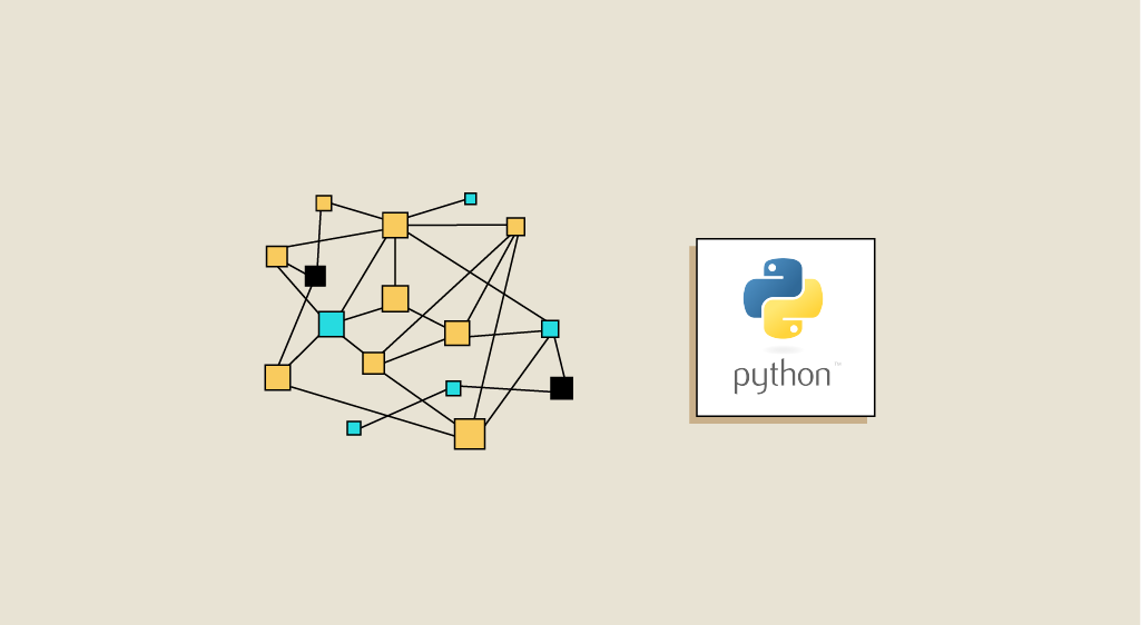
input and output: same colour
middle layers: same colour
example:
The model is made up of an input layer with a number of neurons equivalent to the number of characteristics that a piece of data can have, in our case the number of pixels in an image. You define your input layer using the keras.layers Input constructor, specifying the dimension of our data.
Hidden layers are defined using the Dense constructor, the units argument being used to specify the number of neurons in a layer. For your model, you initialise the first layer with 20 neurons and the second with 14. The two hidden layers will use the relu activation function.
The Output Layer will have a number of neurons equal to the number of distinct classes, in this case the number of digits, i.e. 10.
You will also use the Dense constructor with the softmax function, which gives us a distribution between 0 and 1, which are the probabilities of our data belonging to the respective classes.
This is your model defined after executing the code above.
Compiling the model :
We know you’re dying to get on with training the model, but there’s one last little step we need to take, and that’s to compile our model.
The compile method configures the model training process by specifying 3 important parameters.
- loss: parameter which tells the model which loss function to use to calculate the error and optimise it. Here we’ll use “categorical_crossentropy”.
- optimizer: this parameter defines the optimisation algorithm we are going to use for gradient descent of the loss function. We choose the “adam” optimizer, which generally gives good results on a large set of problems.
- metrics: parameter used to select the model evaluation metrics during the training process. The metric specified for this model is accuracy, the most commonly used metric for classification problems.
- Running the next cell will compile your model and make it ready to be trained.
Model training :
We have finally reached the training phase, where all the magic of Deep Learning takes place. But before we do, there are a few basic concepts that need to be explained.
Deep learning algorithms are known to be fairly data-intensive, with the size of the datasets used to train a neural network reaching hundreds or even thousands of GB, so to enable machines with fairly limited RAM to train models, we divide our dataset into considerably smaller parts called batches so that they can be loaded more easily onto the machine’s RAM.
When all the batches have been run through, an epoch is said to have been completed.
You’ll see that this part isn’t that complicated – in fact, all you need is a single line of code to start training.
However, we’ve promised to explain every detail of the code, so here you’ll run the fit method on your model with your train dataset as arguments and some additional parameters:
- batch_size: the number of data samples a batch will contain
- epoch: the number of epochs required to train the model
- validation_split: the percentage of data that will be used to evaluate our model during training.
The training time for a model can vary according to a number of criteria: the size of the dataset, the complexity of the model architecture, the number of epochs and the computing power.
Evaluation of the model :
Congratulations! You’ve just trained your first Deep Learning model. Now you need to check its performance by measuring its accuracy.
As mentioned above, accuracy is a metric for evaluating classifiers such as the ratio of correctly classified points to the total number of data points.
Running this code will show you the training and validation accuracy as a function of epochs. An example of the results obtained will follow

Training accuracy is obtained by testing with training data, i.e. data that the model has already seen before. Validation accuracy is obtained with new data, which explains the difference in the graph.
Here we have a validation accuracy of 95%, which is a very satisfactory result.
NB: You won’t necessarily get the same results as those displayed because they depend on the random initialisation of the model weights, but the difference won’t be obvious.
Become a Deep Learning pro!
Now that you know how to build, train and test your own neural network, you can dive into the world of Deep Learning and try lots of new things. For this model, you can try modifying the architecture, the activation functions or the training parameters. To do this, take a look at the Keras documentation.
Work on new projects that process data from new and different sources. Don’t limit yourself to just one type of data; tackle structured data and NLP, for example.
And don’t hesitate to keep up to date with our blog, which is packed with knowledge about Deep Learning, like this article, which will expand your theoretical knowledge of the subject.
And if you want to improve your Deep Learning skills, check out the expert courses designed by DataScientest.


