An essential function in Excel, the Dropdown Excel list facilitates data entry on spreadsheets, minimizing errors. But how do you create a drop-down list in Excel? Find out the answers.
What is a Dropdown Excel List?
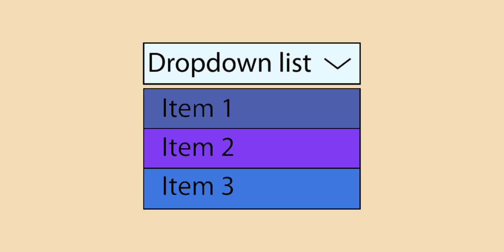
The Dropdown Excel feature that creates a list of predefined choices in a cell. In this way, the user doesn’t need to enter data for each cell. Simply select an option from the drop-down menu.
The Dropdown Excel list is an invaluable tool for data analysts who have to deal with several hundred rows of data. And with good reason, this Excel function enables you to:
- Simplify data entry: thanks to the Dropdown Excel list, you no longer have to enter the same data over and over again. You can simply select the data you need from a list of predefined choices.
- Harmonize data: with manual data entry, you sometimes unintentionally add an accent or an extra space, or make typing errors. The result: multiple entries for a single category. This is no longer the case with the Excel drop-down list, since each entry is made only once, when the list is created.
- Reduce the risk of calculation errors: as the data is uniform, there is less risk of calculation errors.
How do I create a Dropdown Excel list?
There are several ways to create Dropdown Excel list. It all depends on your needs. Here are the main methods.
Simple drop-down list
To create a classic Dropdown Excel list, proceed as follows:
- Select the cells for which you wish to implement the drop-down list;
- Click on “Data”, then “Data validation”;
- In the “Options” tab and the “Allow” zone, select “List”;
- In the “Source” zone, select the relevant cell range;
Click on “OK”.
💡 Related articles:
Drop-down list with fixed values
This type of list is particularly useful if the list values are limited. For example, True/False.
Here’s how it works:
- Select the cells for which you want to implement the drop-down list;
- Click on “Data”, then “Data validation”;
- In the “Options” tab and “Authorize” zone, select “List”;
- In the “Source” zone, select the data to be entered in the list (e.g. TRUE / FALSE);
- Click on “OK”.
Please note! With Excel, typography is crucial, especially when it comes to capitalization. For example, if the user types “true” without capital letters, an error message will appear.
Dropdown Excel list from a named cell range
This type of Dropdown Excel list is particularly useful if your data is going to be modified. With this model, the list will automatically adapt as you add or delete items.
To use this method, you must first name a range of cells. Here’s how to do it:
- Select the cells and click on the “Name box” (above column A);
- Type the name you wish to give to your list (the name must begin with a letter or the “_” sign and contain no spaces).
Then simply create your Dropdown Excel list:
- Select the cells for which you want to implement the drop-down list;
- Click on “Data”, then “Data validation”;
- In the “Options” tab and the “Authorize” zone, select “List”;
- In the “Source” field, type the “=” sign, then the name assigned to your list;
- Click on “OK”.
Dynamic Dropdown Excel list from a table
This is a dynamic list, since the list adapts to any modification of the cell range. In this case, an Excel table.
To do this, you need to name your table. Here’s how to do it:
- Select the entire table or a single cell;
Click on “Table” (in the “Insert” tab); - If you have selected a single cell, Excel will suggest all the cells it considers to be part of the table.
- Check that there are no errors;
- Check the “My table has headers” box;
- Click on “OK”;
- Select the table and click on the “Name zone” (above column A);
- Type the name you wish to give your table.
Then simply repeat the steps for creating a drop-down list in Excel. Namely:
- Select the cells for which you are implementing the drop-down list;
- Click on “Data”, then “Data validation”;
- In the “Options” tab and the “Allow” zone, select “List”;
- In the “Source” field, type “=INDIRECT(“TableName[column header]”) ;
- Click on “OK”.
The Dropdown Excel list, an indispensable tool for data analysts
By facilitating data entry and harmonizing data, the Excel drop-down list simplifies the work of data analysts. This feature lets you enter all types of values (whether fixed cells, tables, etc.). And best of all, with the dynamic drop-down list, any modification to the cell range is automatically integrated.
If you want to master the Excel functions that are useful for data analysis, we invite you to discover our dedicated training course.


