
A Machine Learning model is capable of learning autonomously from one dataset, with the aim of predicting behavior on another dataset. To do this, it finds underlying relationships between independent explanatory variables and a target variable in the initial dataset. It then uses these patterns to predict or classify new data.
How do I define the train_test_split function?
To verify the effectiveness of a Machine Learning model, the initial dataset is divided into two sets: a training set and a test set. The training set is used to fit, i.e. train, the model on part of the data. The test set is used to evaluate the model’s performance on the other part of the data. The train_test_split function in Python’s ScikitLearn (sklearn) library allows this separation into two sets.
First of all, you need to import the train_test_split function from sklearn’s model_selection package using the following code:
Once imported, the function takes several arguments:
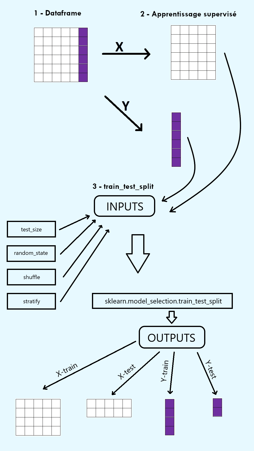
1) Arrays extracted from the dataset to be split.
In supervised learning, these arrays are the input array X, consisting of the explanatory variables in columns, and the output array y, consisting of the target variable (i.e. the labels).
In unsupervised learning, the only array in argument is the input array X, made up of the explanatory variables in columns.
Note: Be careful with dimensions! X must be a two-dimensional array. y must be a one-dimensional array equal to the number of rows in X. To do this, use the .reshape function.
2) Test set size (test_size) and training set size (train_size).
The size of each set is either a decimal number between 0 and 1 representing a proportion of the dataset, or an integer number representing a number of examples in the dataset.
Note: It is sufficient to define just one of these arguments, the second being complementary.
3) The random state (random_state).
The random state is a number that controls how the pseudo-random generator divides the data.
Note: Choosing an integer as the random state ensures that the data is split in the same way each time the function is called. This makes the code reproducible.
4) Le shuffle (shuffle).
Shuffle is a Boolean that selects whether or not data should be shuffled before being separated. If the data is not shuffled, it is separated according to the order in which it was initially displayed.
Note: The default value is True.
5) Stratify (stratify).
The Stratify parameter selects whether the data are separated so as to keep the same proportions of observations in each class in the train and test sets as in the initial dataset.
Remarks:
- This parameter is particularly useful when dealing with “unbalanced” data with very unbalanced proportions between the different classes.
- The default value is None.
The train_test_split function returns a number of outputs equal to twice its number of inputs, in array form. In supervised learning, it returns four outputs: X_train, X_test, y_train and y_test. In unsupervised learning, it returns two outputs: X_train and X_test.
How to evaluate model performance with the train_test_split function?
Once the train_test_split function has been defined, it returns a train set and a test set. This splitting of the data makes it possible to evaluate a Machine Learning model from two different angles.
The model is trained on the train set returned by the function. Then its predictive capabilities are evaluated on the test set returned by the function. Several metrics can be used for this evaluation. In the case of linear regression, the coefficient of determination, RMSE and MAE are preferred. In the case of classification, accuracy, precision, recall and F1-score are preferred. These scores on the test set are therefore used to determine how well the model performs and how much it needs to be improved before it can predict on a new dataset.
The train and test sets returned by the train_test_split function also play an essential role in detecting overfitting or underfitting. As a reminder, overfitting (or overlearning) describes a situation where the model built is too complex (with too many explanatory variables, for example), such that it learns the training data perfectly but fails to generalize to other data.
Conversely, underfitting (or underlearning) describes a situation where the model is too simple or poorly chosen (choosing a linear regression on data that does not respect its assumptions, for example), such that it learns poorly. These two problems can be corrected by various techniques, but they must first be identified, which is made possible by the train_test_split function.
In fact, we can compare the model’s performance on the train set and the test set created by the function. If performance is good on the train set but poor on the test set, we’re probably dealing with overfitting. If performance is as bad on the train set as on the test set, we’re probably dealing with underfitting. The two sets returned by the function are therefore essential in detecting these recurring problems in Machine Learning.
How can I solve a complete Machine Learning problem using the train_test_split function?
Now that we’ve understood the use and functionality of the train_test_split function, let’s put it into practice with a real Machine Learning problem.
Step 1: Understanding the problem
We choose to solve a supervised learning problem where the expected labels are known. More precisely, we focus on binary classification. The objective is to predict whether or not an individual has breast cancer, based on body characteristics.
Step 2: Data recovery
We use the “breast_cancer” dataset included in the Sklearn library.
With the following lines of code, we retrieve the features and the target variable:
We obtain that the target variable to be predicted takes two values (“malignant” and “benign”) and that the problem is indeed a binary classification.
Step 3: Creating X and y
We create a two-dimensional input array X and a one-dimensional output array y. For this dataset, the binary encoding of the target variable is performed by sklearn and can be retrieved directly.
We check that the dimensions of X and y match: y has the same number of rows as X.
Step 4: Creating train and test assemblies
We divide the data into a train set and a test set.
Since we supply the train_test_split function with two arrays X and y, it returns four elements. We choose a test set consisting of 10% of the data. We choose a number of type “int” as the random state to ensure code reproducibility. We don’t use the function’s final parameters, which are unnecessary for such a simple problem.
Step 5: Classification model
To solve the classification task, we build a k-nearest neighbor model. We train the model on the train set using the .fit() method. Then we test the model’s performance on the test set with the .predict() method. This gives us the predicted classes for the observations in the test set.
Step 6: Model evaluation
We choose accuracy as our metric. Accuracy represents the number of correct predictions out of the total number of predictions. We calculate it on the train set and on the test set using the .score() method, which compares the real classes in the dataset with the classes predicted by the clf classifier.
We obtain an accuracy of 0.95 on the train set and 0.93 on the test set. So the model has good classification performance.
What’s more, the accuracy on the test set is very slightly lower than that on the train set. This means that the model generalizes well to new data. So we’re not facing an overfitting problem.
So the train_test_split function is easy to use and highly effective in solving a complete Machine Learning problem.
Are there any limits to the train_test_split function?
Despite this, the train_test_split function has a major limitation linked to its random_state parameter. In fact, when the value given to random state is an integer, the data are separated by a pseudo-random generator initialized with this integer, called seed.
The separation performed is reproducible by keeping the same seed. However, it has been shown that the choice of seed has an influence on the performance of the associated Machine Learning model: different seeds can create different sets and variable scores.
One solution to this problem is to use the train_test_split function several times with different values for the random_state. We can then calculate the average of the scores obtained.
Thus the train_test_split function in the sklearn Python library is essential for conducting a Data Science project and evaluating a Machine Learning model when used properly !


