Neural Style Transfer (NST) is a set of models and methods for transferring the visual style of one image to another, using images or videos. In this article, we’ll be taking a closer look at a particular model called CycleGAN.
Today, the most successful NST algorithms are adapted Deep Learning algorithms using convolution layers. Artistically, NST is most often used to create artificial works of art based on a photograph and a painter’s style. There are currently several applications (mobile and web) for style transfer, such as DeepArt and Reiinakano’s blog. For example, you can transform a Star Wars character (Darth Revan) into a painting inspired by Paul Klee’s Clouds over Bor :

The CycleGAN model, what is it?
As its name suggests, CycleGAN is a type of generative model (created by Jun-Yan Zhu et al. for the BAIR research laboratory at UC Berkeley), a GAN (Generative Adversarial Network) used to perform style transfer on an image. In practice, the vast majority of GANs used to transform an image from the style of a domain X to the style of a target domain Y are trained using a paired dataset in which each image instance of X has an instance directly associated with it in another Y style.
Where CycleGAN stands out is precisely in its lack of need for image peers during training. In fact, when we train such a model, we get very good performance without ever using paired images, which makes training much easier for particular datasets where no correspondence has been made. We can then imitate a painter’s style for different images using a database of his paintings, for example!
First, let’s look at the architecture of a GAN. If you’ve already read one of our articles on GANs, you’ll know that a GAN is a model that breaks down into two large sub-models, a generator and a discriminator:
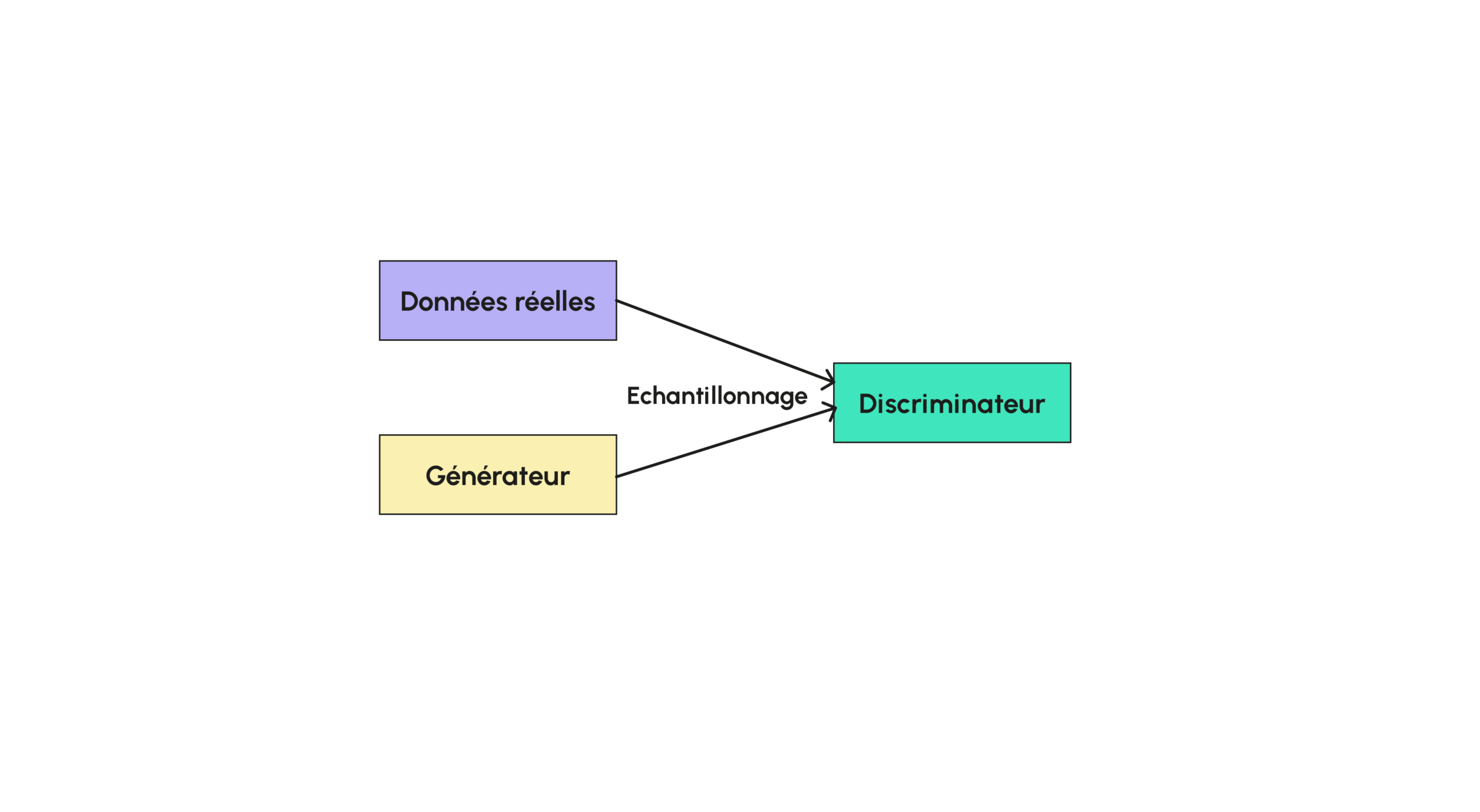
The generator is the model used to generate images, generally from random noise, while the discriminator (which takes a value between 0 and 1) is used to classify a given image to determine whether it is artificial or not. Thus, during training, both the generator and the discriminator are trained so that the discriminator becomes stronger and stronger to differentiate a real image from a generated one, and the generator becomes stronger and stronger to fool the discriminator. During training, the generator does not have direct access to the real data; only the generator uses it to compare with simulated data.
The loss function for the discriminator will be the errors it makes in classifying the data, and that of the generator will be the discriminator’s success in differentiating it from the real images. Some models use the same loss function, which is minimized by the discriminator and maximized by the generator.
The CycleGAN structure is designed so that the generator G translates the distribution from one style X to another style Y, so that the discriminator cannot distinguish the transformed style Y=G(X) from the original style Y. There’s a problem that often arises when applying this strategy as it stands: the generator will translate all the images in the same way, so it can only generate a single example b, which is not the desired task.
To alleviate this problem, the CycleGAN structure will add a constraint by defining another generator F whose role will be to be the inverse transform of G in the sense that FGX≈X. This guarantees that the transformation of X will not be reduced to a single example. A new loss function characterizing cycle consistency loss is therefore added during training, encouraging transformations to verify the properties FGX≈X and that G(FY)≈Y. In addition to the discriminator for G (which we call DY because we want to discriminate Y from Y), we add a discriminator for F (which we call DX). In this paper, we find a diagram summarizing the various relationships described above.
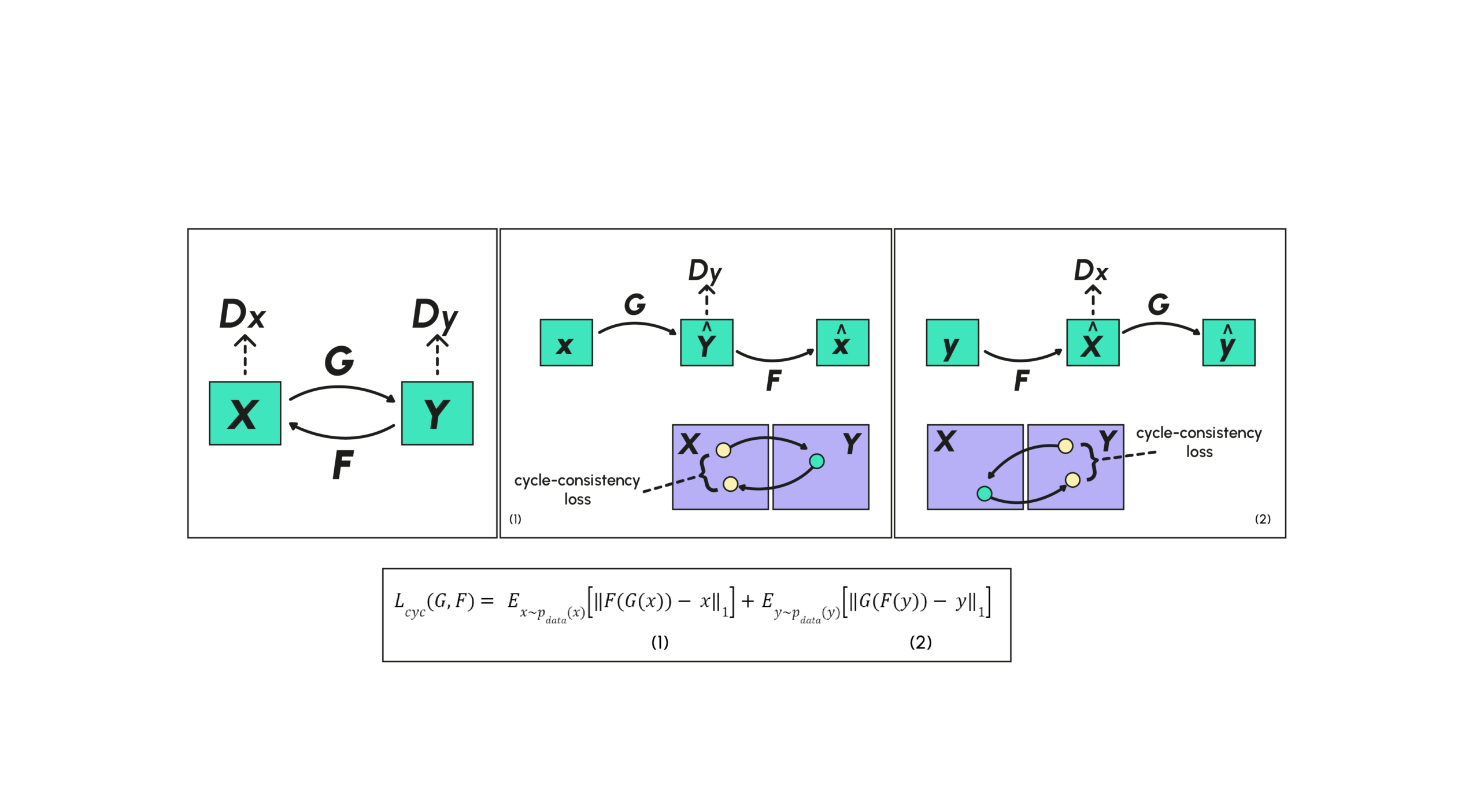
The cycle-consistency loss is then separated into two distinct pieces, the first (1) corresponding to the loss between the elements of X and their reconstructions and the second (2) corresponding to the loss between the elements of Y and their reconstructions.
In this model, the generators and discriminators will optimize the same general loss function, which is made up of two loss sub-functions associated with the generators (adversial loss):


and the cyclic consistency loss function :

giving the overall loss function :

which will be maximized by the discriminators (so that they can distinguish generation from reality) and minimized by the generators, so that they can create examples that are increasingly indistinguishable from real data.
CycleGAN architecture in detail
The two generators and the two discriminators are perfectly identical in architecture, i.e. they are made up of the same layers and have the same dimensions. The generators mainly use convolution layers and residual blocks.
The convolution layers have already been discussed and explained in detail in another article on our blog, which you can find here.
Residual blocks are very simple layers in Deep Learning, often used in style transfer, which ensure that the image doesn’t stray too far from the original one, recalling it to the network as it goes along. More formally, such a layer is of the form :
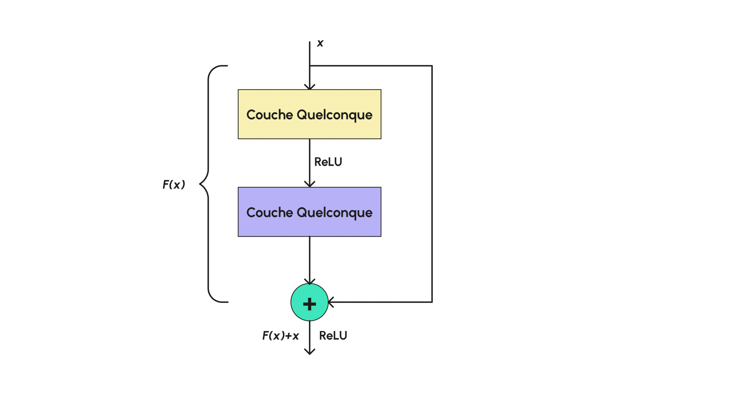
So, as shown in graph (d), the residual block just consists of a normal layer, to which the initial input value is added at the end.
A ReLU is also applied in some cases, to cancel the layer output if F(x) turns out to be too high negatively (where a color image would have positive values).
For discriminators, the model uses 70 x 70 PatchGANs, i.e. the discriminator will be made up of several small GANs, PatchGANs of initial size 70 x 70, which will be applied all over the image and may overlap in the part of the image under consideration, determining whether a given part of the image is real or not.
The final response is then calculated as the average of the responses returned for each patch. Each PatchGAN will have a similar architecture consisting solely of classical convolution layers. Finally, training is performed with a batch size of 1 and a classical optimizer: Adam.
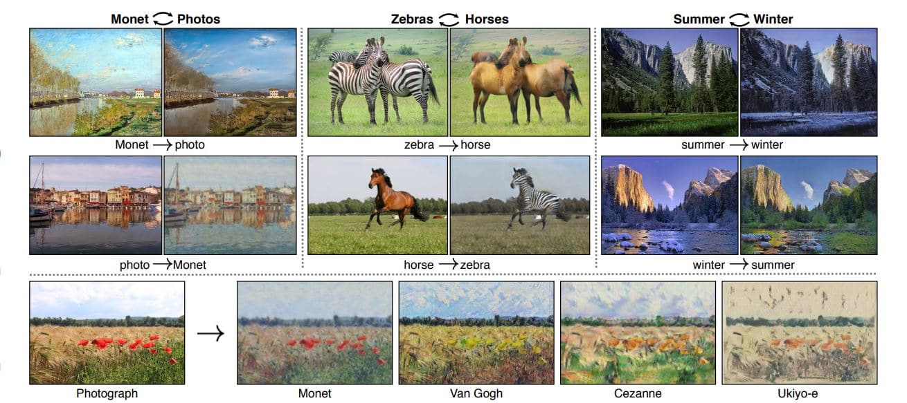
Here we present some results obtained with test images through the previously defined model; on the left we have the original images provided as input and on the right the transfigured images. We can see, for example, that the model trained with images of horses and zebras can switch freely from one animal style to the other.
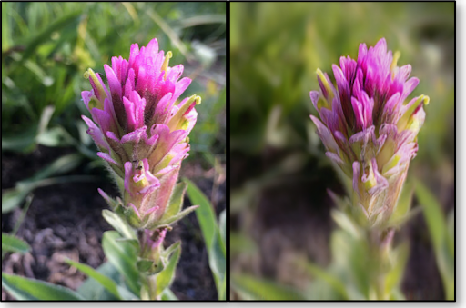
Similarly, when trained with artists’ paintings, it can switch from a photograph to a painting in the style of Van Gogh. Very good results are also obtained in image reconstruction. In addition to the near-identical reconstruction, the quality of the reconstructed image is improved (with better depth of field) compared with the basic image:
In this article, we looked at what style transfer is, and more specifically at the architecture of the CycleGAN model, inspired by GANs, for efficient style transfer. CycleGAN is one of the best algorithms for style transfer. We have also seen that this algorithm, unlike almost all style transfer algorithms, does not require matched data, which is complicated to obtain in practice, and can therefore be used to train different databases that were previously unusable, such as those of paintings by famous painters like Van Gogh.
Finally, we have seen that in addition to efficient style transfer, this model also features faithful image reconstruction, resulting in an output image with a better-realized depth of field, demonstrating the algorithm’s stability. This algorithm is not all-powerful, however, as it has shortcomings when it comes to modifying the geometric properties of images, such as when you want to turn a cat into a dog, so it is only suitable for changing textures.
If you’d like to learn more about object transfiguration, Deep Learning and artificial intelligence applied to images, take a look at our Data Scientist training course.

